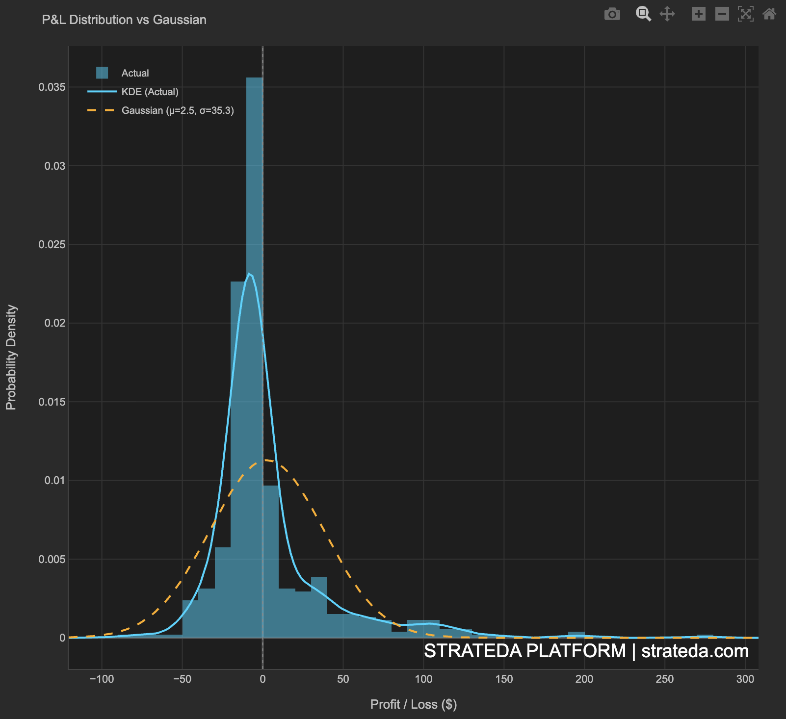
P&L vs Gaussian (Fat-Tail Detection)

What it is

This view overlays your actual trade return distribution with a theoretical Gaussian (normal) distribution that has the same mean and standard deviation. The comparison reveals whether your returns have fat tails — extreme outcomes that occur more often than a normal distribution predicts. Fat tails matter because they mean your worst (and best) outcomes will be larger and more frequent than standard risk metrics assume.

Most financial return distributions have fat tails. The question is how fat, and whether the tails are symmetric or one-sided. This directly affects how much you should trust standard deviation and Sharpe ratio as risk measures.

How to access it

Navigate to the P&L vs Gaussian tab in the performance dashboard. Available on Plus and above.

What you see

• Histogram — Your actual trade P&L distribution.
• KDE curve — A smooth kernel density estimate of your actual distribution.
• Gaussian overlay — An orange dashed curve fitted to your data's mean and standard deviation, labelled in the legend as 'Gaussian (μ=X, σ=Y)' where X and Y reflect the actual values from your trade set.
• Overlap and divergence areas — Where the actual distribution exceeds the Gaussian (fat tails) and where it falls below (thinner center or different peak).
• Legend — Identifies three elements: 'Actual' (the histogram bars), 'KDE (Actual)' (the smooth cyan curve), and 'Gaussian (μ=X, σ=Y)' (the orange dashed reference curve).

The two curves share the same center and width, so differences are purely about shape — particularly in the tails.

How to interpret it

Skewness

• Positive skew (> 0.5) — Right tail is longer. You have occasional large wins that pull the mean above the median. Typical of trend-following and momentum strategies. Win rate may be below 50%, but the large wins compensate.
• Near zero (−0.5 to 0.5) — Roughly symmetric. Wins and losses are similar in magnitude. Typical of well-calibrated crossover strategies.
• Negative skew (< −0.5) — Left tail is longer. You have occasional large losses that pull the mean below the median. Typical of mean-reversion and premium-selling strategies. Win rate is often high, but blow-up risk exists.

Kurtosis

• Low kurtosis (< 3) — Thin tails. Extreme outcomes are rare. Returns behave close to normal.
• High kurtosis (> 3) — Fat tails. Extreme outcomes (both positive and negative) occur more often than a normal distribution predicts. This is common in financial returns and means you should not rely on standard deviation alone for risk measurement.

Distribution shape vs. strategy type

Shape	Typical strategy	Concern if unexpected
Positive skew, low win rate	Trend following, breakout	If you expect mean-reversion, your exits may be wrong
Symmetric, moderate win rate	Crossover, momentum	Expected shape — verify skewness matches backtest
Negative skew, high win rate	Mean reversion, selling premium	Large-loss tail is your primary risk — monitor closely

Tail behavior

Actual distribution exceeds Gaussian in the tails: Fat tails confirmed. You experience extreme wins and/or extreme losses more often than a normal model predicts. Standard risk metrics (VaR based on normal distribution, Sharpe ratio interpretation) underestimate your true risk. Expect occasional outsized moves in both directions.

Actual distribution exceeds Gaussian in one tail only: Asymmetric fat tail. If the left tail is fatter (more extreme losses than expected), you have hidden downside risk. If the right tail is fatter (more extreme wins), your strategy captures outlier moves — a positive trait for trend-following strategies.

Actual distribution matches the Gaussian closely: Rare but possible with some well-diversified or high-frequency strategies. Standard risk metrics are reliable. You can use normal-distribution-based position sizing with more confidence.

Actual distribution has a taller, narrower peak than the Gaussian: Leptokurtic distribution — most trades cluster tightly around the mean, but the tails are heavier. This is the classic financial return shape. Most days are normal; the occasional day is extreme.

Practical implications

• For position sizing: If your tails are fatter than Gaussian, use more conservative position sizing than standard formulas suggest. The "3-sigma event" that standard models say is rare will happen more often than once every 370 trades.
• For stop-loss placement: Fat left tails mean your worst-case losses are larger than standard deviation implies. Set stop-losses based on actual maximum adverse excursion (see MAE vs MFE), not on multiples of standard deviation.
• For expectation setting: Fat right tails mean occasional windfall trades. Don't increase position size based on a few large wins — they're real but infrequent.

Example

P&L vs Gaussian for 200 trades on a DEMA/EMA crossover on EURCHF:

• Actual distribution: Positive mean (+$4.12), skewness +1.24, kurtosis 4.8.
• Gaussian fit: Same mean and standard deviation, kurtosis 3.0 (by definition).

Visual comparison:

• The actual distribution has a slightly taller peak than the Gaussian — more trades cluster near the mean than a normal distribution predicts.
• The right tail extends further — a handful of trades returned 3–4× the average win. The Gaussian predicts almost zero probability at those levels.
• The left tail is slightly heavier than Gaussian but less pronounced than the right tail — the distribution is asymmetrically fat-tailed.

Interpretation: The strategy produces returns that are more concentrated around the mean than normal (most trades are "typical"), but with occasional outsized wins that a Gaussian model doesn't predict. The rightward skew is favorable — tail risk is biased toward large wins, not large losses. Standard Sharpe ratio underestimates the strategy's quality because it penalizes the positive tail equally with the negative one.