Backtest Metrics Reference

What it is

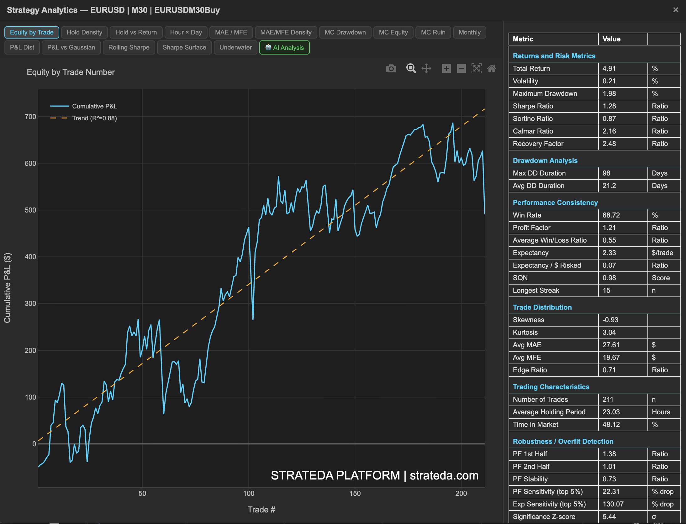
The single backtest metrics table provides a complete statistical picture of your strategy's performance. It is accessed via the table icon on any loaded equity curve in the View Panel. The metrics are grouped into seven sections — each answering a specific question about your strategy.

This page is a reference for every metric in the table. Use it to look up definitions, understand units, and interpret values. For guidance on reading the equity curve, trade log, and trade markers, see Backtesting. For the full analytics dashboard with charts and visualizations, see Backtest Analytics.

How to access it

After a backtest completes, the equity curve appears in the View Panel. The metrics are displayed in a persistent panel on the right side of the Strategy Analytics popup — always visible alongside whichever analytics tab is active on the left. Click the table icon on the loaded curve in the View Panel to open the Strategy Analytics popup. Available on all plans — some advanced metrics require Plus and above.

The metrics popup is accessed via the table icon in the View Panel. See The Strategy Panel & View System for full details.

What you see

Section 1 — Returns and Risk Metrics

Core performance and risk-adjusted return measures.

Metric	Description	Unit
Total Return	Net return over the full backtest period	%
Volatility	Annualised standard deviation of returns	%
Maximum Drawdown	Largest peak-to-trough decline	%
Sharpe Ratio	Return per unit of volatility (annualised, risk-free rate = 0)	Ratio
Sortino Ratio	Like Sharpe but only penalises downside volatility — rewards strategies that have upside variability without downside risk	Ratio
Calmar Ratio	Annualised return divided by maximum drawdown — measures return relative to worst-case pain	Ratio
Recovery Factor	Total return divided by maximum drawdown — how many times over the strategy recovered its worst loss	Ratio

Section 2 — Drawdown Analysis

How long and how deep drawdowns last.

Metric	Description	Unit
Max DD Duration	Longest time spent in drawdown (peak to recovery) — the longest you would have waited to see a new equity high	Days
Avg DD Duration	Average drawdown duration across all drawdown periods	Days

Section 3 — Performance Consistency

Win rate, expectancy, and streak measures that reveal whether the strategy's edge is consistent or dependent on a few trades.

Metric	Description	Unit
Win Rate	Percentage of trades that closed with a profit	%
Profit Factor	Gross profit divided by gross loss — above 1.0 means gross wins exceed gross losses	Ratio
Average Win/Loss Ratio	Average winning trade size divided by average losing trade size	Ratio
Expectancy	Average expected profit per trade in dollar terms — the mean P&L across all trades	$/trade
Expectancy / $ Risked	Expectancy normalised by average amount risked per trade — how much you earn per dollar risked	Ratio
SQN	System Quality Number — combines expectancy and trade count into a single quality score. Above 2.0 is good; above 3.0 is excellent	Score
Longest Streak	Longest consecutive winning streak	n

Section 4 — Trade Distribution

Statistical shape of your trade-level returns — skewness, kurtosis, and trade excursion measures.

Metric	Description	Unit
Skewness	Asymmetry of the return distribution. Positive = right tail (occasional large wins). Negative = left tail (occasional large losses)	—
Kurtosis	Fat-tail measure. Above 3 indicates more extreme outcomes than a normal distribution predicts	—
Avg MAE	Average Maximum Adverse Excursion — how far trades moved against you before closing	$
Avg MFE	Average Maximum Favourable Excursion — how far trades moved in your favour before closing	$
Edge Ratio	MFE divided by MAE — above 1.0 indicates trades move further in your favour than against you. Higher is better	Ratio

Section 5 — Trading Characteristics

How the strategy trades — frequency, holding period, and market exposure.

Metric	Description	Unit
Number of Trades	Total completed trades in the backtest period. More trades provide more statistical confidence — below 30 trades, most metrics are unreliable	n
Average Holding Period	Mean time a position is held open	Hours
Time in Market	Percentage of total backtest period with an open position — reveals whether the strategy is mostly in or mostly out of the market	%

Section 6 — Robustness / Overfit Detection

Tests that assess whether the strategy's edge is genuine, consistent, and not dependent on a few outlier trades.

Metric	Description	Unit
PF 1st Half	Profit factor calculated on the first half of trades	Ratio
PF 2nd Half	Profit factor calculated on the second half of trades	Ratio
PF Stability	Ratio of PF 2nd Half to PF 1st Half. Above 0.8 indicates consistent performance across the backtest period. Below 0.5 suggests the edge is decaying or was front-loaded	Ratio
PF Sensitivity (top 5%)	How much profit factor drops when the top 5% of winning trades are removed. High values indicate dependence on outlier wins — the strategy's profitability may rely on a few large trades	% drop
Exp Sensitivity (top 5%)	How much expectancy drops when the top 5% of winning trades are removed	% drop
Significance Z-score	Z-score testing whether returns are statistically different from zero. Above 1.65 = 90% confidence, above 1.96 = 95% confidence	σ
Significance P-value	Probability that results occurred by chance. Below 0.05 is the standard significance threshold — less than 5% chance the returns are random	—
Regime Consistency	How consistently the strategy performs across thirds of the backtest period (e.g., 2/3 means profitable in 2 of 3 periods, 3/3 means all three)	thirds

Section 7 — Monte Carlo (1000 simulations)

Probabilistic risk assessment from 1000 resampled trade sequences — reveals the range of outcomes you could experience with the same trades in different orders.

Metric	Description	Unit
MDD 50th pctile	Median maximum drawdown across 1000 resampled trade sequences — the drawdown you should expect on a typical run	%
MDD 95th pctile	Worst-case maximum drawdown at 95th percentile — your realistic worst case. Use this for position sizing and capital planning	%
Sharpe CI (90%)	90% confidence interval for the Sharpe ratio — the range of likely true Sharpe values given trade variability	—
Expectancy CI	90% confidence interval for expectancy per trade	$
PF CI (90%)	90% confidence interval for profit factor	—
P(Ruin above 10%)	Probability of a 10% account drawdown occurring across 1000 simulations	%
P(Ruin above 20%)	Probability of a 20% account drawdown occurring	%
P(Ruin above 30%)	Probability of a 30% account drawdown occurring	%

---

Metric Formulas

Every formula below is extracted directly from the platform's Python calculation engine. All metrics operate on the closed-trade record for the backtest period unless stated otherwise.

---

Returns and Risk Metrics

---

Total Return

             E_final − E_start
R_total  =  ──────────────────  ×  100
                  E_start

Where:

• E_final = equity after the last closed trade
• E_start = starting balance as configured in the strategy

Platform convention: Expressed as a percentage. Uses the last valid equity value to handle backtests where the final trade may still be open at evaluation time.

---

Volatility

σ_daily  =  std(r_d)  ×  100

where the daily return series is constructed as:

         E_d − E_(d−1)
r_d  =  ──────────────
            E_(d−1)

Where:

• E_d = equity at the end of calendar day d, sampled by resampling the trade-close equity series to daily frequency and forward-filling days with no closed trades
• r_d = daily percentage return
• std() = sample standard deviation (ddof = 1)

Platform convention: Reported as daily volatility (not annualised), expressed as a percentage. Forward-fill is applied to days with no trade closures. The annualised form (σ_daily × √252) is used internally for ratio calculations but is not displayed as a standalone metric.

---

Maximum Drawdown

                   E_t − peak_t
MDD  =  | min_t ( ──────────── ) |  ×  100
                     peak_t

  where  peak_t = max(E_s)  for all s ≤ t

Where:

• E_t = equity after the t-th closed trade
• peak_t = running peak equity up to trade t

Platform convention: Expressed as a positive percentage. Computed on the trade-close equity series — intrabar equity dips between trade closures are not captured.

---

Sharpe Ratio

          R_ann
SR  =  ─────────
         σ_ann

  where:
    R_ann      =  (R_total / 100)  ×  (252 / T_trading)
    σ_ann      =  (σ_daily / 100)  ×  √252
    T_trading  =  T_calendar  ×  (252 / 365)

Where:

• R_total = Total Return (%)
• σ_daily = daily volatility (%)
• T_calendar = calendar days from first trade open to last trade close
• T_trading = T_calendar scaled to trading days

Platform convention: Risk-free rate = 0. Annualisation uses a calendar-to-trading-day scaling factor of 252/365. Volatility is derived from daily equity returns with forward-fill on days with no closed trades.

---

Sortino Ratio

              R_ann
Sortino  =  ─────────
              σ_down

  where:
    σ_down  =  std( only r_d where r_d < 0 )  ×  √252

Where:

• Only daily returns where r_d < 0 are included in σ_down
• R_ann = annualised return (same as Sharpe)

Platform convention: Risk-free rate = 0. Downside deviation uses only days with negative returns. Returns ∞ when there are no negative daily returns (infinite Sortino).

---

Calmar Ratio

              R_ann
Calmar  =  ───────────
            MDD / 100

Where:

• R_ann = annualised return (same as Sharpe)
• MDD = Maximum Drawdown (%)

Platform convention: Uses the same 252/365 annualisation convention as Sharpe and Sortino. Returns 0 when maximum drawdown is zero.

---

Recovery Factor

         R_total
RF  =  ───────────
           MDD

Where:

• R_total = Total Return (%)
• MDD = Maximum Drawdown (%)

Platform convention: Dimensionless ratio — both inputs are in percentage points so the scaling cancels. Returns ∞ when MDD = 0.

---

Performance Consistency

---

Win Rate

        number of winning trades
W%  =  ────────────────────────────  ×  100
                   N

Where:

• N = total number of closed trades
• A winning trade has profit > 0

Platform convention: Breakeven trades (profit = 0 exactly) are counted as losses.

---

Profit Factor

        Σ( winning trade P&Ls )
PF  =  ────────────────────────────
        | Σ( losing trade P&Ls ) |

Where:

• Numerator = gross profit: sum of all winning trade P&Ls
• Denominator = gross loss: absolute sum of all losing trade P&Ls

Platform convention: Returns ∞ when there are no losing trades. Operates on raw dollar P&L.

---

Average Win/Loss Ratio

        mean( profit_wins )
WL  =  ─────────────────────────
        | mean( profit_losses ) |

Where:

• profit_wins = mean P&L across winning trades
• profit_losses = mean P&L across losing trades

Platform convention: Returns ∞ when there are no losing trades. Distinct from Profit Factor: WL compares averages; PF compares totals.

---

Expectancy

E  =  (W/N × w̄)  −  (L/N × l̄)

Where:

• W = number of winning trades, L = number of losing trades
• N = total trades
• w̄ = mean P&L of winning trades, l̄ = mean absolute P&L of losing trades

Platform convention: Expressed in dollars per trade.

---

Expectancy / $ Risked

E_R  =  (W/N × w̄/l̄)  −  L/N

Where:

• W/N = win rate as a decimal, L/N = loss rate as a decimal
• w̄ = mean winning P&L, l̄ = mean absolute losing P&L

Platform convention: Dimensionless ratio. Returns ∞ when there are no losing trades.

---

SQN (System Quality Number)

          μ_P
SQN  =  ─────  ×  √N
          σ_P

Where:

• μ_P = mean trade P&L across all N trades
• σ_P = standard deviation of trade P&L (ddof = 1)
• N = total number of closed trades

Platform convention: Van Tharp's original formulation operating on raw dollar P&L. Returns 0 when N ≤ 1 or σ_P = 0.

---

Trade Distribution

---

Skewness

                √( N(N−1) )
g₁  =  γ₁  ×  ─────────────
                   N − 2

          (1/N) × Σ(Pᵢ − P̄)³
γ₁  =  ──────────────────────────
        [ (1/N) × Σ(Pᵢ − P̄)² ]^(3/2)

Where:

• P_i = P&L of trade i, P̄ = mean trade P&L, N = number of trades

Platform convention: Computed via scipy.stats.skew() with bias correction (Fisher–Pearson). Positive = right-tailed (occasional large wins). Negative = left-tailed (occasional large losses).

---

Kurtosis

                 (1/N) × Σ(Pᵢ − P̄)⁴
Kurt_excess  =  ──────────────────────────  −  3
                [ (1/N) × Σ(Pᵢ − P̄)² ]²

Where:

• P_i, P̄, N = same as Skewness above

Platform convention: Returns excess kurtosis (Fisher definition: normal distribution = 0, not 3). Values above 0 indicate fat tails relative to a normal distribution. Note: the P&L vs Gaussian chart interprets kurtosis on this same scale — values above 0 indicate heavier tails than normal, not values above 3.

---

Edge Ratio

         mean(MFE)
ER  =  ─────────────
         mean(MAE)

  where for each trade i:
    MFE_i  =  max(E_t) − E_t_open    (max over bar closes while trade is open)
    MAE_i  =  E_t_open − min(E_t)    (min over bar closes while trade is open)

Where:

• E_t = equity at bar close time t
• t_open, t_close = trade open and close timestamps

Platform convention: Excursions are computed from bar-close equity, not from bar high/low prices. ER > 1.0 means trades move further in your favour than against you on average.

---

Robustness / Overfit Detection

---

PF Stability

                  min(PF_1, PF_2)
PF_Stability  =  ─────────────────
                  max(PF_1, PF_2)

Where:

• PF_1 = Profit Factor on the first ⌊N/2⌋ trades (chronological)
• PF_2 = Profit Factor on the remaining trades

Platform convention: Result is always in [0, 1]. Returns ∞ when either half contains no losing trades.

---

PF Sensitivity

                        PF_reduced
PF_Sensitivity  =  (1 − ────────────)  ×  100
                        PF_original

  where:
    k  =  max(1, ⌊0.05 × N⌋)

Where:

• k = number of best trades removed (minimum 1, maximum 5% of N)
• PF_original = Profit Factor over all N trades
• PF_reduced = Profit Factor after removing the top k winning trades

Platform convention: Expressed as percentage drop in Profit Factor when the best 5% of trades are excluded. Returns ∞ when N < 20.

---

Significance Z-score

        p̂ − 0.5
Z  =  ─────────────
        √(0.25 / N)

Where:

• p̂ = observed win rate as a decimal (W / N)
• N = total number of trades
• 0.5 = null hypothesis win rate (random strategy)

Platform convention: One-sample Z-test for the binomial proportion. Tests whether observed win rate is significantly above 50%. Requires no normality assumption on trade P&L — only that trades are independent.

---

Significance P-value

p  =  1 − Φ(Z)

Where:

• Φ(·) = standard normal CDF
• Z = Significance Z-score as defined above

Platform convention: One-tailed p-value testing win rate > 50%. Tests only win rate — use alongside Expectancy and Profit Factor for a complete picture.

---

note

All trade P&L values are raw dollar amounts. For strategies with variable position sizing, metrics that depend on average or total P&L (Profit Factor, Expectancy, SQN, Edge Ratio) reflect the combined effect of signal quality and sizing decisions and cannot be attributed to signal quality alone.

How to interpret it

Reading the sections together

The seven sections build a complete picture when read in sequence:

1. Returns and Risk tell you the headline numbers — what the strategy returned and at what cost.
2. Drawdown Analysis tells you how painful the journey was — not just the depth of losses but how long they lasted.
3. Performance Consistency tells you whether the edge is reliable trade-to-trade or dependent on win rate vs. win size.
4. Trade Distribution reveals the statistical shape — are there fat tails, and do trades move further in your favour than against you?
5. Trading Characteristics tell you how the strategy operates — is it always in the market or selective?
6. Robustness is the most important section for deployment decisions — it tests whether the edge is genuine, consistent, and not dependent on outliers.
7. Monte Carlo gives you probabilistic risk bounds — what could happen with the same trades in a different order.

Key thresholds for deployment readiness

Metric	Deployable	Caution	Redesign
Sharpe Ratio	Above 1.0	0.5–1.0	Below 0.5
Profit Factor	Above 1.3	1.0–1.3	Below 1.0
PF Stability	Above 0.8	0.5–0.8	Below 0.5
PF Sensitivity (top 5%)	Below 20%	20–40%	Above 40%
Significance P-value	Below 0.05	0.05–0.10	Above 0.10
Regime Consistency	3/3	2/3	1/3
Edge Ratio	Above 1.0	0.7–1.0	Below 0.7
P(Ruin above 20%)	Below 5%	5–15%	Above 15%

Example

Backtest metrics for a DEMA/EMA crossover on EURCHF M30 over 12 months (200 trades):

Returns and Risk:

• Total Return: +8.1%, Volatility: 12.4%, Max Drawdown: −4.2%
• Sharpe: 1.14, Sortino: 1.52, Calmar: 1.93, Recovery Factor: 1.93

Drawdown: Max DD Duration: 18 days, Avg DD Duration: 6 days

Consistency:

• Win Rate: 76%, Profit Factor: 1.48, W/L Ratio: 0.62
• Expectancy: +$4.12/trade, SQN: 2.8, Longest Streak: 11

Trade Distribution:

• Skewness: +1.24, Kurtosis: 4.8
• Avg MAE: $8.40, Avg MFE:$12.20, Edge Ratio: 1.45

Trading Characteristics:

• Trades: 200, Avg Holding: 14.2 hours, Time in Market: 42%

Robustness:

• PF 1st Half: 1.52, PF 2nd Half: 1.44, PF Stability: 0.95
• PF Sensitivity: 18%, Exp Sensitivity: 22%
• Z-score: 2.14, P-value: 0.016, Regime Consistency: 3/3

Monte Carlo:

• MDD 50th: −3.8%, MDD 95th: −7.2%
• Sharpe CI: 0.72–1.56, PF CI: 1.18–1.82
• P(Ruin above 10%): 3.2%, P(Ruin above 20%): 0.1%

Interpretation: This strategy passes all key thresholds. PF Stability of 0.95 confirms the edge is consistent across the full backtest period. Low PF Sensitivity (18%) means the strategy doesn't depend on outlier wins. The P-value of 0.016 provides strong statistical significance. Monte Carlo worst-case drawdown (95th percentile) of −7.2% is manageable, and the probability of a 20% ruin event is near zero. The strategy is ready for walk-forward validation.