WFO Metrics Reference

What it is

The WFO Summary Statistics table consolidates the most important walk-forward metrics into a single view. Rather than navigating through individual charts to piece together a picture, this table answers the key questions immediately: How many windows were profitable? How much did performance degrade from IS to OOS? Are the results statistically significant?

Each section of the table addresses a specific dimension of walk-forward quality — from basic window profitability through to statistical robustness. Together, they provide the fastest path to a GO/NO-GO decision on whether a strategy is ready for deployment.

How to access it

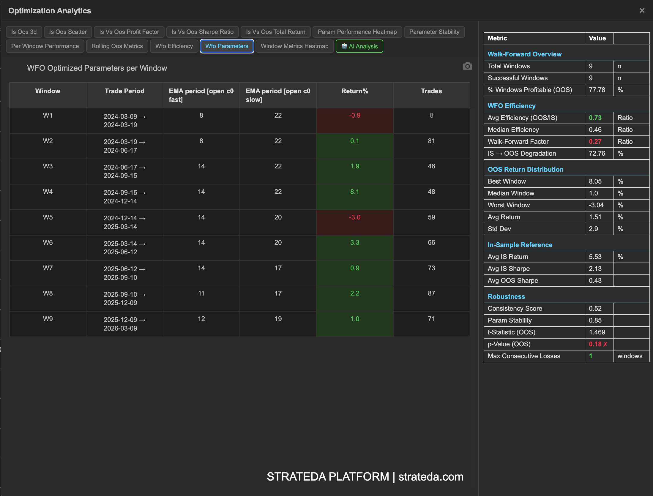
The WFO Summary Statistics table is accessed via the global table icon at the bottom of the View Panel when a WFO result is loaded. Loading a WFO result clears all previously loaded curves and displays the combined OOS equity curve. Clicking the table icon opens the WFO analytics popup — the Summary Statistics table is the first view.

Available on Premium plans. The optimization analytics popup is accessed via the table icon in the View Panel after your WFO job completes. See The Strategy Panel & View System for full details.

tip

Use this table as your first stop after a WFO run — it gives you a GO/NO-GO signal before diving into the individual analytics charts. A strategy passing the key thresholds here (above 60% profitable windows, Walk-Forward Factor above 0.3, p-Value below 0.10) warrants deeper analysis. One that fails multiple thresholds should be redesigned before going live.

What you see

The table is divided into five sections, each answering a different question about your walk-forward results.

Walk-Forward Overview

Basic counts and success rates across all WFO windows.

Metric	Description
Total Windows	Total number of WFO windows configured and run. More windows provide more statistical power — see Walk-Forward Optimization for guidance on window count.
Successful Windows	Number of windows that completed without errors. Should equal Total Windows unless data gaps or computation issues occurred.
% Windows Profitable (OOS)	Percentage of out-of-sample windows that produced positive returns. This is the single most intuitive WFO metric — it tells you how often the re-optimized strategy made money on unseen data.

WFO Efficiency

How much of the in-sample performance survives contact with out-of-sample data.

Metric	Description
Avg Efficiency (OOS/IS)	Average ratio of OOS return to IS return across all windows. A value of 0.6 means the strategy retains 60% of its in-sample performance out-of-sample. Values above 0.5 are shown in green — the strategy retains more than half its IS edge.
Median Efficiency	Middle efficiency value across all windows. Less affected by outlier windows (one very good or very bad OOS period) than the average. Compare to Avg Efficiency — if they diverge significantly, outlier windows are skewing the average.
Walk-Forward Factor	Overall OOS/IS return ratio across the entire test period (not per-window, but aggregate). This is the headline efficiency number. See WFO Efficiency Ratio for detailed interpretation.
IS→OOS Degradation	Percentage drop from average IS return to average OOS return. Calculated as (IS − OOS) / IS × 100%. Lower is better. Some degradation is expected and healthy — the optimizer had the advantage of fitting to IS data.

OOS Return Distribution

Statistical summary of out-of-sample returns across all windows — how your strategy performed on data it never saw during optimization.

Metric	Description
Best Window	Highest OOS return achieved across all windows. Shows the upper bound of forward-tested performance.
Median Window	Median OOS return across all windows. The most representative single number for "what to expect" from a typical OOS window.
Worst Window	Lowest OOS return across all windows — can be negative. This is the realistic downside scenario for any single deployment period.
Avg Return	Mean OOS return across all windows. Compare to Median Window — if the mean is significantly higher, a few strong windows are pulling the average up.
Std Dev	Standard deviation (population) of OOS returns across windows. Lower means more consistent window-to-window performance. High standard deviation means OOS outcomes are unpredictable even if the average is positive.

In-Sample Reference

Baseline IS metrics that provide context for evaluating OOS performance. These are what the optimizer achieved on the data it was fitted to — the ceiling your OOS results are measured against.

Metric	Description
Avg IS Return	Average in-sample return across all windows. This is the theoretical best-case — what the optimizer found when it had the advantage of seeing the data.
Avg IS Sharpe	Average in-sample Sharpe ratio across all windows. The risk-adjusted IS benchmark.
Avg OOS Sharpe	Average out-of-sample Sharpe ratio across all windows. Compare directly to Avg IS Sharpe to assess quality degradation — not just return degradation, but risk-adjusted degradation. A strategy that drops from IS Sharpe 2.0 to OOS Sharpe 1.0 has degraded significantly in return but may still be deployable.

Robustness

Statistical measures that assess whether the WFO results are genuine or could have occurred by chance.

Metric	Description
Consistency Score	The Sharpe ratio of window-level OOS returns — mean OOS return divided by the standard deviation of OOS returns across windows. Higher values indicate more consistent performance relative to variability. Values above 0.5 indicate reliable consistency; values below 0 mean the average OOS window was unprofitable.
Param Stability	Measures how stable the selected parameters are across windows on a 0–1 scale. Above 0.75 indicates the optimizer consistently finds similar parameters — it's detecting the same market pattern each time. Below 0.5 suggests regime-dependent parameters where the optimizer finds different "best" values in each window. Values below 0 indicate extreme parameter instability where parameters vary by more than 100% of their mean value. See Parameter Stability for the full visual analysis.
t-Statistic (OOS)	Tests whether mean OOS returns are significantly different from zero using a one-sample t-test with df = N−1 degrees of freedom. Critical values depend on the number of windows — use the p-Value directly for significance assessment as it already accounts for the correct degrees of freedom automatically.
p-Value (OOS)	Probability that the observed OOS results occurred by chance. Below 0.10 is the practitioner-grade threshold — less than a 10% chance the results are random. Below 0.05 is the institutional standard. Values are shown in red when above the threshold (e.g., 0.18 ✗) as a visual warning. This is a two-tailed test — p < 0.10 here is equivalent to a one-tailed test at p < 0.05 for assessing one-directional profitability.
Max Consecutive Losses	Maximum number of consecutive losing OOS windows. This measures the worst streak your strategy experienced during walk-forward testing. 1–2 consecutive losses is normal and expected. 3+ warrants investigation — check whether those windows correspond to a specific market regime using the OOS Metrics Heatmap.

Metric Formulas

Every formula below is extracted directly from compute_wfo_metrics(). All calculations operate on the list of successfully completed window analytics entries.

For formulas covering Total Return, Sharpe Ratio, and Profit Factor per window see Backtest Metrics Reference.

---

% Windows Profitable

                # windows where OOS total_return > 0
% Profitable = ──────────────────────────────────────── × 100
                           N_windows

Variables:

• N_windows = number of successfully completed OOS windows
• OOS total_return = Total Return (%) for each window's out-of-sample period

Platform convention: Strictly greater than zero. Breakeven windows count as unprofitable.

---

Avg Efficiency and Median Efficiency

Per-window efficiency:

           OOS_return_w
  eff_w = ──────────────    for each window w where |IS_return_w| > 0.001
           IS_return_w

  Avg Efficiency    = mean({ eff_w })
  Median Efficiency = median({ eff_w })

Variables:

• OOS_return_w = OOS total return (%) for window w
• IS_return_w = IS total return (%) for window w
• 0.001 = minimum IS return threshold to prevent division instability

Platform convention: Each window contributes equally to the average regardless of IS magnitude. Compare to Walk-Forward Factor which weights by IS magnitude.

---

Walk-Forward Factor

         Σ OOS_return_w
  WFF = ────────────────────    where |Σ IS_return_w| > 0.001
         Σ IS_return_w

Variables:

• Σ OOS_return_w = sum of all OOS returns across windows (%)
• Σ IS_return_w = sum of all IS returns across windows (%)

Platform convention: Unlike Avg Efficiency, computed on aggregate totals — windows with larger IS returns have proportionally more influence. This is the single headline number for overall IS-to-OOS retention.

---

IS→OOS Degradation

                    r̄_OOS
  Degradation = (1 − ────── ) × 100
                    r̄_IS

              = ( r̄_IS − r̄_OOS ) / r̄_IS  ×  100

Variables:

• r̄_IS = mean IS total return across all windows (%)
• r̄_OOS = mean OOS total return across all windows (%)

Platform convention: Expressed as a percentage. Lower values are better. Returns None when |mean IS return| ≤ 0.001.

---

OOS Return Distribution (Best / Median / Worst / Avg / Std Dev)

  Best   = max({ OOS_return_w })
  Median = median({ OOS_return_w })
  Worst  = min({ OOS_return_w })
  Avg    = mean({ OOS_return_w })

             ┌──────────────────────────────────────────────────┐
             │  1                                            2   │
  Std Dev = √│ ─── × Σ ( OOS_return_w − mean(OOS_return) )     │
             │  N                                               │
             └──────────────────────────────────────────────────┘

Variables:

• { OOS_return_w } = set of OOS total returns across all N windows (%)
• N = number of completed windows

Platform convention: Std Dev uses population standard deviation (divides by N, not N−1). All five metrics operate on the same OOS return series.

---

Avg IS Return / Avg IS Sharpe / Avg OOS Sharpe

  Avg IS Return  = mean({ IS_return_w })
  Avg IS Sharpe  = mean({ IS_sharpe_w })
  Avg OOS Sharpe = mean({ OOS_sharpe_w })

Variables:

• IS_return_w = IS total return for window w (%)
• IS_sharpe_w = IS annualised Sharpe ratio for window w — see Backtest Metrics Reference
• OOS_sharpe_w = OOS annualised Sharpe ratio for window w

Platform convention: Equal-weight averages — each window contributes once regardless of length. IS metrics are the theoretical ceiling against which OOS is measured.

---

Consistency Score

              mean({ OOS_return_w })
  CS  =  ────────────────────────────
              std({ OOS_return_w })

Variables:

• { OOS_return_w } = OOS returns across all completed windows (%)
• std(·) = population standard deviation (ddof = 0)

Platform convention: This is the Sharpe ratio of window-level OOS returns. It is NOT bounded to [0, 1]:

• Above 1.0 → mean return is large relative to variability
• 0.5 to 1.0 → reliable consistency
• 0 to 0.5 → moderate consistency
• Below 0 → mean OOS return was negative

Returns None when Std Dev = 0 or N ≤ 1.

---

Param Stability

Step 1 — Coefficient of Variation per parameter:

              std({ param_value_w })
  CV_p  =  ──────────────────────────    for each optimized parameter p
            | mean({ param_value_w }) |

Step 2 — Stability Score:

  Param Stability  =  1  −  mean({ CV_p })

Variables:

• { param_value_w } = selected values of parameter p across all windows
• std(·) = population standard deviation (ddof = 0)
• CV_p = coefficient of variation for parameter p (dimensionless)

Platform convention: Only parameters that vary across windows and have a non-zero mean are included.

  Near 1.0  → parameters nearly constant across all windows
  ≈ 0.75    → moderate stability (avg CV ≈ 0.25)
  ≈ 0.50    → high variability (avg CV ≈ 0.50)
  Below 0   → extreme instability (parameters vary > 100% of their mean)

---

t-Statistic (OOS)

        r̄_OOS × √N
  t  = ─────────────    df = N − 1
              s

Variables:

• r̄_OOS = mean OOS return across N windows (%)
• s = sample standard deviation of OOS returns (ddof = 1)
• N = number of completed windows
• df = degrees of freedom for the t-distribution

Platform convention: Computed via scipy.stats.ttest_1samp(oos_returns, 0). This is a two-tailed test. Critical values depend on df and are higher than z-distribution thresholds for typical WFO window counts:

  N windows | df | t for p<0.10 | t for p<0.05
  ──────────┼────┼──────────────┼─────────────
       5    |  4 |     2.13     |     2.78
       6    |  5 |     2.02     |     2.57
       7    |  6 |     1.94     |     2.45
       8    |  7 |     1.90     |     2.37
       9    |  8 |     1.86     |     2.31
      10    |  9 |     1.83     |     2.26

Use the p-Value directly for significance assessment — it accounts for the correct degrees of freedom automatically.

---

p-Value (OOS)

  p  =  P( |T_df| ≥ |t_observed| )    ← two-tailed

Variables:

• t_observed = t-Statistic as defined above
• df = N − 1
• N = number of completed windows

Platform convention: Two-tailed p-value from scipy.stats.ttest_1samp(). Because this is a two-tailed test, p < 0.10 here is equivalent to a one-tailed test at p < 0.05 for assessing one-directional profitability.

  p < 0.05   ✓   Strong evidence — institutional standard
  p < 0.10   ~   Practitioner threshold
  p ≥ 0.10   ✗   Insufficient evidence

Returns None when N < 3.

---

Max Consecutive Losses

  Algorithm (chronological order):
    current ← 0,  max ← 0
    for each OOS_return_w:
      if OOS_return_w < 0:
        current ← current + 1
        max ← max(max, current)
      else:
        current ← 0
    return max

Variables:

• OOS_return_w = OOS total return for window w in chronological order

Platform convention: Strictly less than zero. A window returning exactly 0.00% breaks the streak.

How to interpret it

Quick assessment framework

Read the table top to bottom. Each section builds on the previous:

1. Walk-Forward Overview answers: "Did the basic test work?" — If % Windows Profitable is below 50%, stop here.
2. WFO Efficiency answers: "How much edge survived?" — Walk-Forward Factor below 0.1 means almost nothing survived optimization.
3. OOS Return Distribution answers: "What should I actually expect?" — Median Window is your best single estimate of per-window live performance.
4. In-Sample Reference answers: "How much did I lose from theory to reality?" — Compare IS Sharpe to OOS Sharpe for the clearest picture.
5. Robustness answers: "Can I trust these results?" — p-Value below 0.10 and Param Stability above 0.75 together provide strong evidence.

Key thresholds

Metric	Deployable	Caution	Redesign
% Windows Profitable	> 60%	50–60%	< 50%
Walk-Forward Factor	> 0.3	0.1–0.3	< 0.1
IS→OOS Degradation	< 50%	50–80%	> 80%
Consistency Score	> 0.5	0–0.5	< 0
Param Stability	> 0.75	0.5–0.75	< 0.5
p-Value (OOS)	< 0.05	0.05–0.10	> 0.10
Max Consecutive Losses	1–2	3	4+

A strategy that passes all "Deployable" thresholds has strong evidence behind it. A strategy in the "Caution" range on 1–2 metrics may still be deployable at reduced position size. A strategy hitting "Redesign" on multiple metrics should not be deployed — revisit the strategy logic, indicator selection, or parameter ranges.

Example

WFO Summary Statistics for a DEMA/EMA crossover on EURCHF M30 with 9 windows:

Walk-Forward Overview:

• Total Windows: 9
• Successful Windows: 9
• % Windows Profitable: 66.7% (6 of 9)

WFO Efficiency:

• Avg Efficiency: 0.52 (green)
• Median Efficiency: 0.48
• Walk-Forward Factor: 0.47
• IS→OOS Degradation: 53%

OOS Return Distribution:

• Best Window: +4.2%
• Median Window: +1.1%
• Worst Window: −2.8%
• Avg Return: +1.3%
• Std Dev: 2.1%

In-Sample Reference:

• Avg IS Return: +2.8%
• Avg IS Sharpe: 1.82
• Avg OOS Sharpe: 0.85

Robustness:

• Consistency Score: 0.61
• Param Stability: 0.78
• t-Statistic (OOS): 1.86
• p-Value (OOS): 0.07 ✓
• Max Consecutive Losses: 2

Interpretation: This strategy passes all key thresholds. 66.7% of windows are profitable (above 60%). The Walk-Forward Factor of 0.47 indicates the strategy retains nearly half its IS performance — moderate but genuine. IS→OOS degradation of 53% is in the caution range but the absolute OOS Sharpe (0.85) is still meaningfully positive. The p-Value of 0.07 falls below the 0.10 practitioner threshold, and Param Stability of 0.78 confirms the optimizer is finding the same market pattern across windows. Max Consecutive Losses of 2 is within normal bounds.

This strategy is deployable. The summary statistics suggest deploying at moderate position size with ongoing monitoring — the edge is real but not overwhelming, and the trader should watch for OOS Sharpe deterioration as evidence of potential regime change.