Parameter Heatmaps (2D Sharpe Grid)
What it is
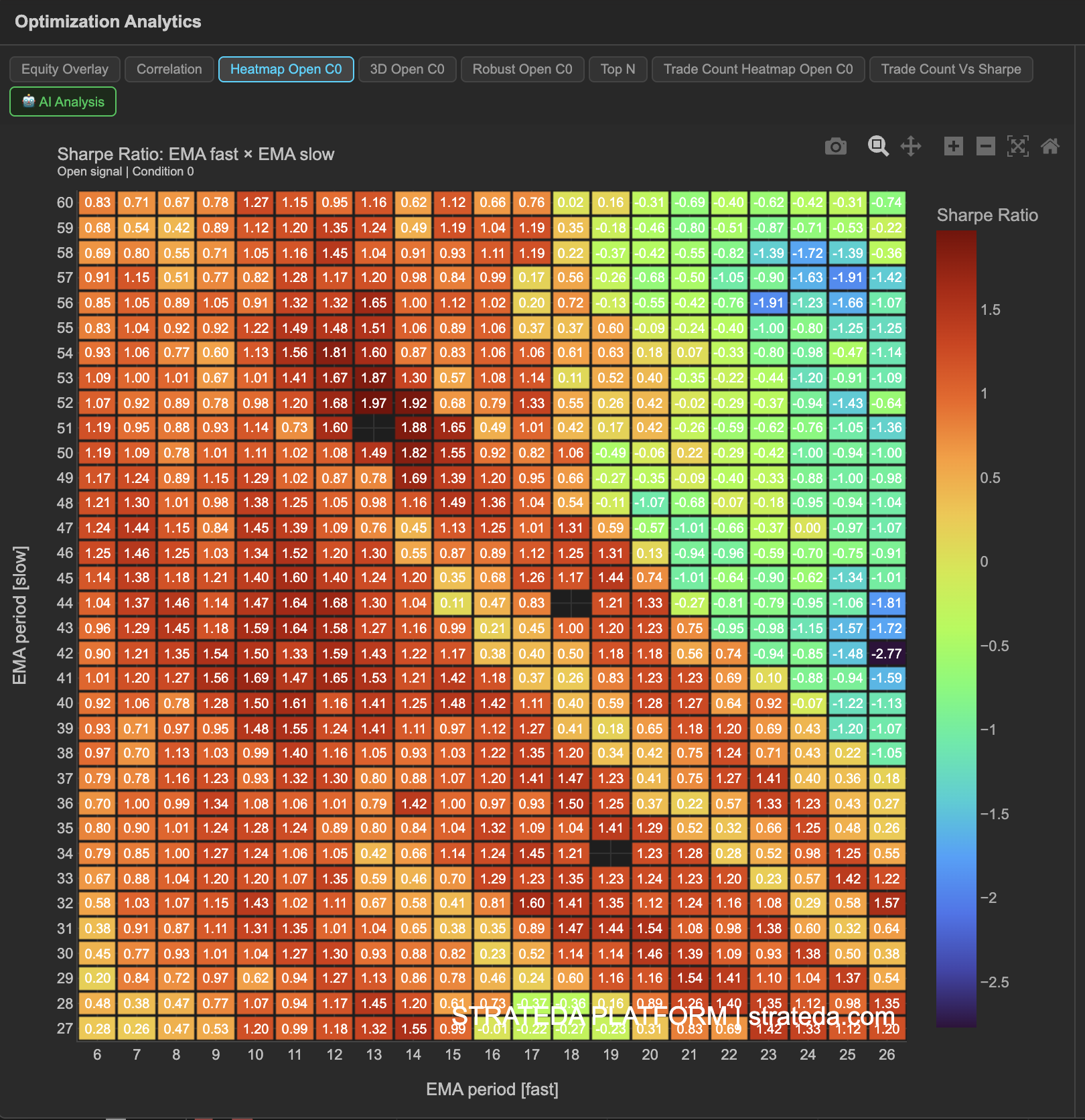
The Parameter Heatmap displays a color-coded 2D grid where each cell represents one parameter combination and its color intensity corresponds to the Sharpe ratio (or another selected metric). With one parameter on each axis, you can instantly see which regions of the parameter space perform well and which don't — without reading through a table of hundreds of rows.
This is one of the most useful optimization views because it reveals structure in the results. A single "best" number tells you nothing about whether that result is stable. A heatmap shows you whether good performance is clustered in a region (robust) or isolated to a single cell (fragile).
How to access it
Navigate to the Heatmap Open C0 tab in the optimization analytics popup. Available on Plus plans and above. The "Open C0" label refers to the Open signal, Condition 0 — the first condition of your open signal.
The optimization analytics popup is accessed via the table icon in the View Panel after your optimization job completes. See The Strategy Panel & View System for full details.
What you see
- X-axis — Values of the first optimized parameter (e.g., EMA period: 5, 10, 15, ..., 65).
- Y-axis — Values of the second optimized parameter (e.g., DEMA period: 5, 10, 15, ..., 65).
- Cell color — Intensity represents the Sharpe ratio for that specific combination. Warm colors (yellow, orange) indicate higher Sharpe; cool colors (blue, purple) indicate lower or negative Sharpe.
- Cell values — The exact Sharpe ratio is displayed within each cell or available on hover.
For a 20 × 20 optimization, the heatmap contains 400 cells — the full parameter landscape at a glance.
How to interpret it
What good looks like:
- A broad region of warm-colored cells (high Sharpe) clustered together. This means neighboring parameter values produce similar results — the strategy is not sensitive to exact parameter choices in that area.
- The warm cluster is not at the extreme edges of your tested range. Edge results suggest the optimal parameters might be outside your range entirely.
What bad looks like:
- A single bright cell surrounded by cold cells. This is the classic sign of overfitting — one combination happened to fit the data, but slight parameter changes destroy performance.
- A random scattershot of warm and cold cells with no visible pattern. This suggests the strategy has no meaningful relationship between parameter values and performance — results are likely noise.
- All cells are cold (low or negative Sharpe). The strategy concept doesn't work well for any parameter combination on this instrument and timeframe.
Practical guidance:
- Choose parameters from the center of a warm cluster, not the single hottest cell. Center-of-cluster parameters are more likely to generalize to unseen data.
- If the warm region sits at the edge of your grid, consider expanding your optimization range in that direction.
Example
A heatmap for a DEMA × EMA crossover optimization on BTC shows:
- A warm cluster in the EMA 25–45 / DEMA 10–25 region, with Sharpe ratios between 1.0 and 1.8.
- The single highest Sharpe (1.82) is at EMA 35 / DEMA 15, but its neighbors (EMA 30/DEMA 15, EMA 35/DEMA 20) also score above 1.4.
- The lower-left corner (short periods for both) shows negative Sharpe — fast crossovers generate too many false signals on this instrument.
- The upper-right corner (long periods for both) shows near-zero Sharpe — signals are too infrequent for meaningful results.
The trader selects EMA 35 / DEMA 15 with confidence, knowing it sits in a stable region rather than being an isolated peak.