Walk-Forward Optimization: How to Know When Your Strategy Works — and When to Stop
Estimated reading time: 35 minutes
Introduction
Walk-forward optimization is the most rigorous method available for testing whether a trading strategy has a real, repeatable edge, or whether it merely memorized a particular stretch of historical data. Standard backtesting has a fundamental flaw, when you optimize parameters on a dataset and then measure performance on the same dataset, you are selecting the best-fitting parameters after seeing all outcomes. Given enough combinations, some will appear excellent purely by chance. Walk-forward optimization breaks this cycle by testing each set of optimized parameters on data the optimizer has never seen.
The result is not a prediction. It is a probabilistic model of a non-stationary dynamic system, with empirical evidence for its time of validity and observable signals for when the model is no longer valid. Systematic trading does not offer certainty. It offers calibrated probabilities, honest risk boundaries, and a framework for making deployment decisions based on evidence rather than hope.
This report applies that framework to a concrete case study, a long-only EMA crossover strategy on BTCUSD M30, developed step by step from an initial backtest through parameter optimization, quality filtering, and walk-forward validation across 5 and 11 rolling windows. The central finding is that the strategy demonstrates a statistically significant edge in the current BTC market regime, remains profitable during the declining price phase of 2025 to 2026 that was entirely unseen during optimization, and reveals a clear regime boundary at late 2023 that separates two structurally different periods of market behavior.
The report is organized as follows. Chapter 1 establishes the baseline backtest and its limitations. Chapter 2 describes the parameter optimization process and the overfitting problem it exposes. Chapter 3 adds a quality filter and confirms a robust parameter region. Chapter 4 presents the primary walk-forward validation across 5 windows. Chapter 5 extends the analysis to 11 windows and identifies the regime boundary. Chapter 6 establishes a Monte Carlo risk framework for live deployment. The conclusion synthesizes all findings into a deployment hypothesis and a framework for ongoing strategy management.
1. Baseline Backtest
Method
The strategy under analysis is a long-only EMA crossover on BTCUSD M30. The entry signal fires when the fast EMA crosses above the slow EMA. The exit signal fires when the fast EMA crosses back below the slow EMA. No stop-loss, no take-profit, and no additional filters are applied at this stage. Position sizing is fixed at 20% margin on a $10,000 account, meaning $2,000 of margin is deployed per trade.
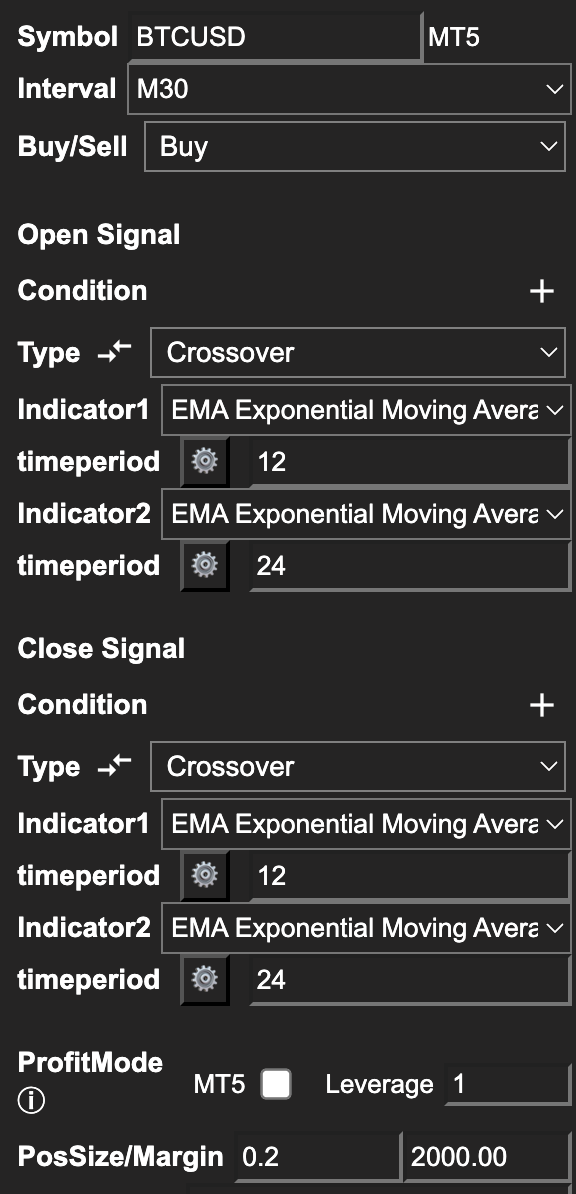
Figure 1: Strategy Builder showing EMA(12)/EMA(24) crossover setup on M30
The instrument and timeframe were chosen deliberately. BTCUSD provides a long history of varied market regimes, including sustained bull markets, sharp bear markets, and extended ranging periods, all within a single instrument. This regime diversity makes it a meaningful test bed for walk-forward validation methodology. The M30 timeframe generates enough trades per 6-month period to produce statistically interpretable metrics in each walk-forward window, which matters when configuring the validation step later.
Starting parameters are EMA(12) as the fast line and EMA(24) as the slow line. These were chosen as intuitive starting values, not as optimized parameters. The purpose of this chapter is to establish a reference point before any optimization takes place.
The backtest is run on MT5-connected broker data via the Strateda MT5 integration, covering January 2024 to March 2026. This period was selected because it represents the most recent 2+ years of data available at the time of writing and forms the foundation period for all subsequent optimization work.
Results
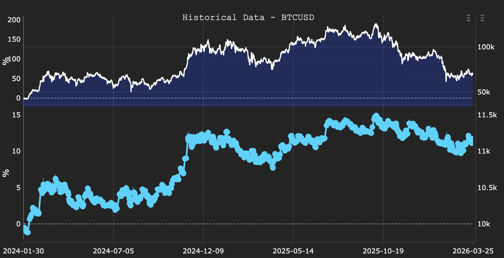
Figure 2: BTCUSD price and equity overlay January 2024 to March 2026
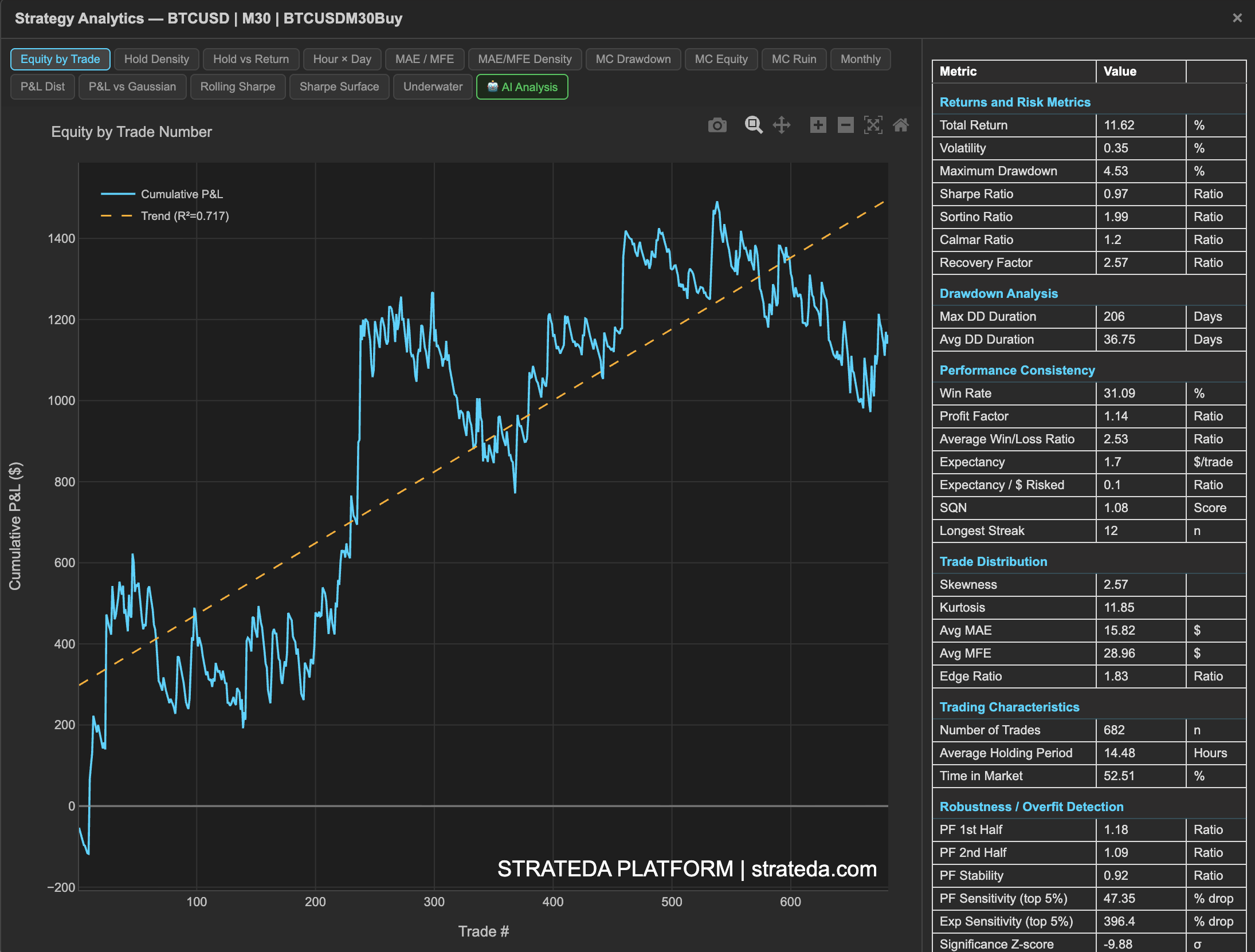
Figure 3: Strategy Analytics showing equity curve and full metrics table
Description of Results
The backtest produces a total return of 11.62% over the 2.4-year period, with a Sharpe ratio of 0.97, a maximum drawdown of 4.53%, and 682 trades. The win rate is 31.09%, the profit factor is 1.14, and the average win/loss ratio is 2.53. The equity curve trends upward with a regression R² of 0.717, indicating a moderately consistent upward trajectory with meaningful deviations from the trend line.
The upper chart shows the BTCUSD price history alongside the strategy equity curve. The lower chart shows the full metrics table alongside the equity curve plotted against trade number. The trend line and R² value quantify how consistently the strategy generated returns across the full period.
One observation from the price and equity overlay deserves attention. BTC price peaked at approximately +200% gain before retracing to approximately +50% by period end, giving back roughly 75% of its peak gain. The strategy equity peaked at approximately +15% and ended at +11.62%, giving back approximately 23% of its peak gain. The strategy is not simply tracking BTC price in both directions. It captured a significant portion of the upside and preserved the majority of its gains during the retracement phase.
Interpretation
The numbers are positive but not compelling in isolation. A Sharpe ratio below 1.0, a win rate of 31%, and a profit factor of only 1.14 indicate a strategy with a thin edge at these default parameters. The low win rate combined with a win/loss ratio of 2.53 confirms this is a momentum-style strategy, most trades are small losses, but the winners are significantly larger, producing a net positive expectancy per trade.
The bull market context must be acknowledged honestly. This backtest covers January 2024 to March 2026, a period that includes one of the strongest sustained Bitcoin bull runs in history. A long-only strategy of almost any kind will produce positive results during this period. However, the asymmetry between BTC's peak-to-end retracement and the strategy's retracement is early evidence that the exit mechanism is functioning as designed. The absolute return of 11.62% is less important than this shape. Position size can scale the return up or down.
Conclusion
The baseline establishes that the strategy concept is viable at default parameters. It produces positive returns, manageable drawdowns, a trade count sufficient for further analysis, and early evidence of downside protection relative to passive BTC exposure. A single in-sample backtest on a trending period is not validation of a real edge. The next step is to explore the parameter space systematically and understand where genuine signal exists.
2. Parameter Optimization
Method
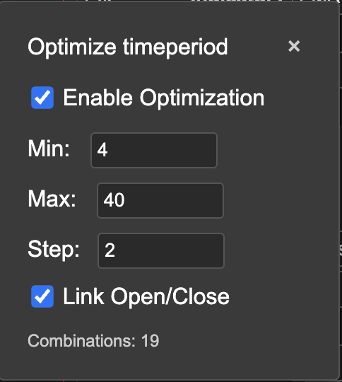
Figure 4: Fast EMA range setup, min 4, max 40, step 2
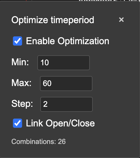
Figure 5: Slow EMA range setup, min 10, max 60, step 2
Parameter optimization runs a systematic grid search across a defined range of parameter values, backtesting every combination independently and ranking the results by a chosen metric. This maps the full performance landscape of the parameter space rather than relying on a single intuitive starting point.
The optimization is run on an in-sample period from January 2024 to March 2025, approximately 15 months. This period was chosen deliberately to reflect current market conditions rather than older data from structurally different market phases. The fast EMA range is set from 4 to 40 with a step of 2, generating 19 values. The slow EMA range is set from 10 to 60 with a step of 2, generating 26 values, for a total of 476 combinations. Combinations are ranked by Sharpe ratio with a minimum trade count filter of 70.
Results
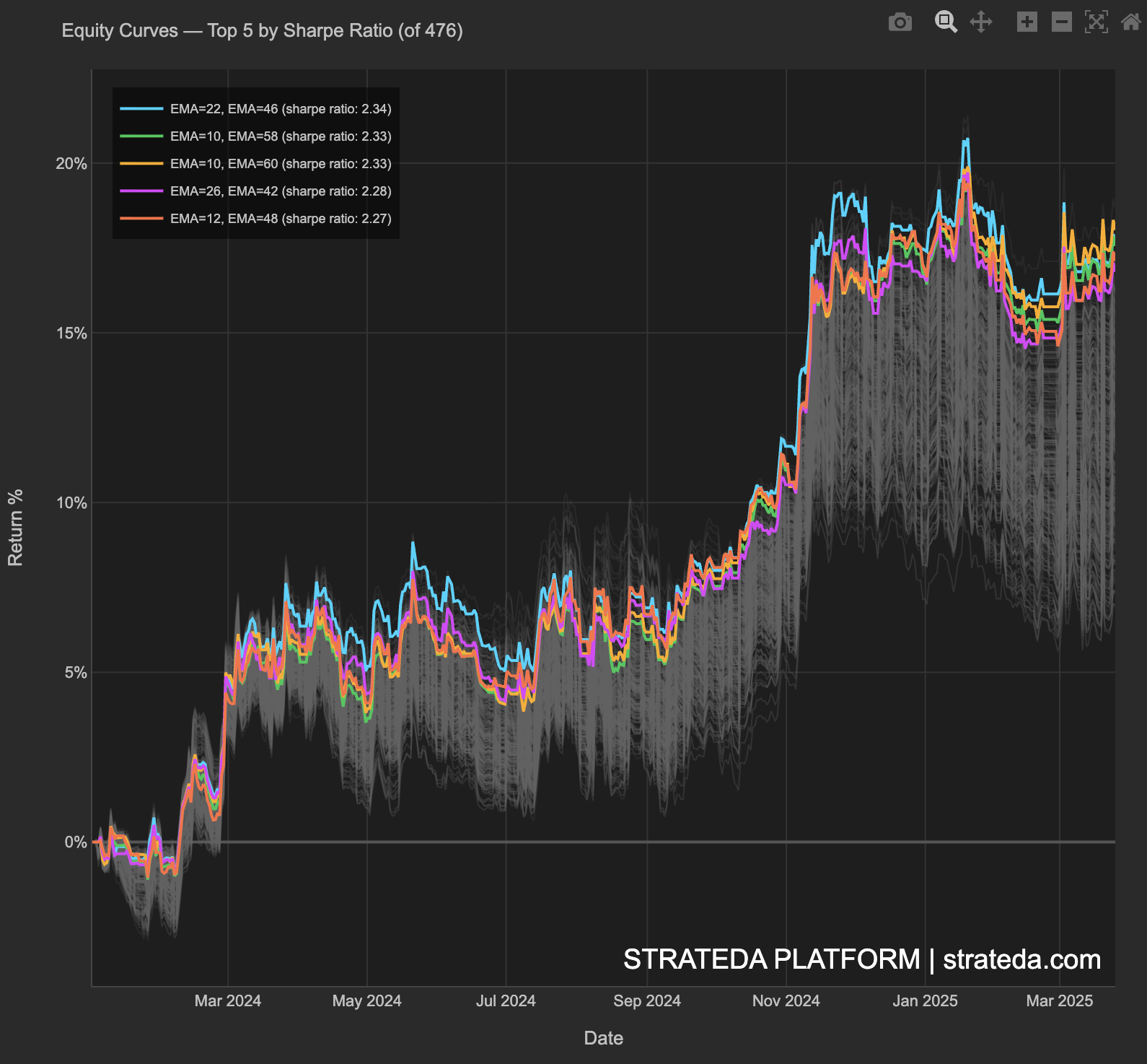
Figure 6: Equity Curves showing Top 5 by Sharpe Ratio of 476 combinations
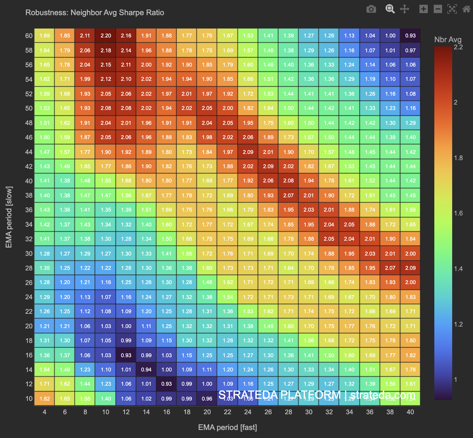
Figure 7: Robustness heatmap from optimization run without RSI filter.
Description of Results
The equity curve fan plots all 476 combinations simultaneously, with the top 5 by Sharpe ratio highlighted in color and all others rendered in gray. The top combination is EMA(22, 46) with Sharpe 2.34, followed closely by EMA(10, 58) and EMA(10, 60) at Sharpe 2.33. The colored lines pull clearly away from the gray mass, suggesting the top combinations outperform the median result by a meaningful margin.
The robustness heatmap shows two distinct high-performance regions. The first is in the upper-left at fast EMA 6 to 10 combined with slow EMA 54 to 60, reaching neighbor-averaged Sharpe above 2.1. The second is in the lower-right at fast EMA 28 to 40 combined with slow EMA 28 to 44, reaching similar values. The weakest region sits in the middle of the grid around fast 12 to 16 and slow 14 to 22, where the two EMAs are closest together and generate excessive conflicting signals. This two-zone structure is the key finding from the broad optimization, the parameter landscape is not a single smooth peak but two distinct robust regions separated by a poor-performing valley.
Interpretation
The robustness heatmap reveals two distinct high-performance zones separated by a cold valley in the middle of the grid. This two-zone structure is not what a pure bull market effect would produce. A market that simply rewarded any long strategy would show a uniformly warm grid. Instead, the cold region around fast 12 to 16 and slow 14 to 22, where the two EMAs are closest together, shows that parameter choice matters. The optimizer is finding real structure in the data, not just confirming that BTC went up.
The two robust zones define the candidate parameter ranges for the next step. The upper-left zone at fast 6 to 10 and slow 54 to 60 represents a wide-gap configuration where the slow EMA acts as a long-term trend filter. The lower-right zone at fast 28 to 40 and slow 28 to 44 represents a tighter, faster configuration. Both survive neighbor averaging, meaning neither depends on an exact parameter combination to produce strong results.
Conclusion
The optimization identified two distinct high-performance zones in the robustness heatmap. The first is a stripe at fast EMA 6 to 10 with slow EMA 54 to 60. The second is a diagonal stripe at fast EMA 28 to 40 with slow EMA 28 to 44. Rather than selecting either stripe, the WFO parameter ranges were chosen to cover the quadratic region between them, fast EMA 6 to 20 and slow EMA 40 to 62.
A quadratic region is preferable to a stripe for walk-forward optimization. A stripe indicates robustness along one parameter axis only, meaning the optimizer has limited flexibility when re-optimizing on new IS data. A quadratic region maintains consistent performance across both parameter dimensions, giving the WFO optimizer a stable two-dimensional target to land in regardless of how market conditions shift the optimal values within the window.
3. Quality Filter and Robustness Confirmation
Method
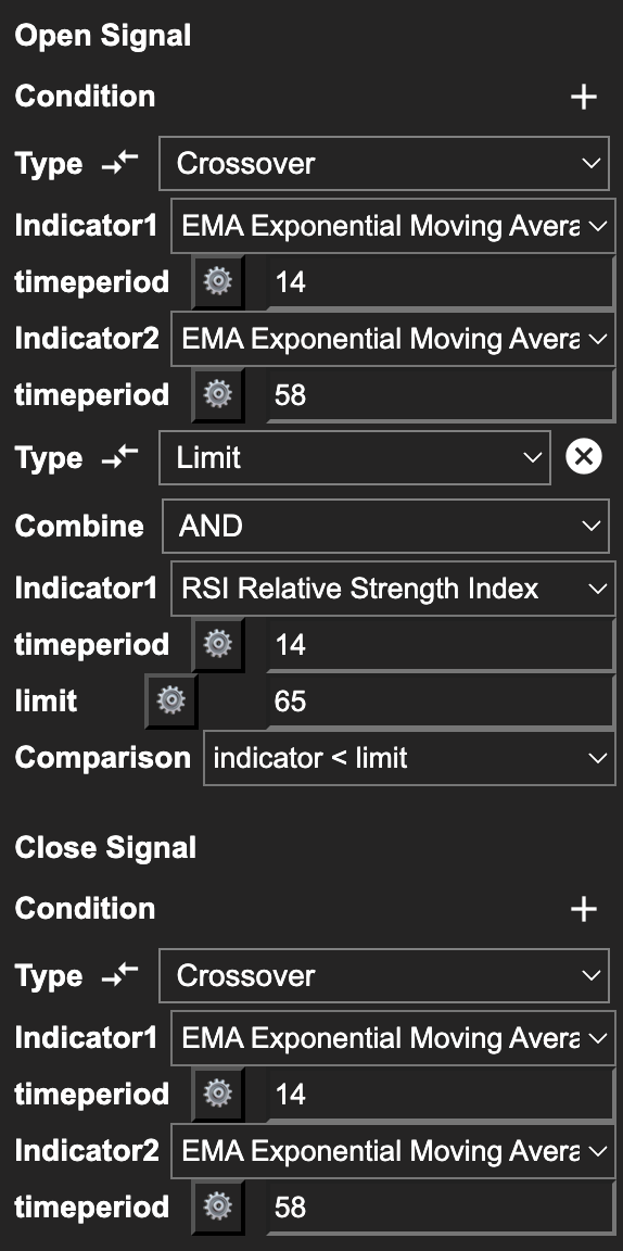
Figure 8: Strategy Builder showing EMA crossover with RSI(14) filter added as AND condition
The bare EMA crossover enters on every crossover regardless of market context. A crossover signal when BTC is already overbought is less reliable than one that fires while momentum is still building. Adding a quality filter restricts entries to a more favorable subset of signals by requiring a secondary condition to be met alongside the crossover.
The filter is an RSI(14) limit condition added to the entry signal with AND logic. The strategy only enters long when the fast EMA crosses above the slow EMA and the RSI is simultaneously below the limit value. Four limit values are tested 50, 55, 60, and 65. The RSI period of 14 is fixed and not optimized.
With the RSI limit confirmed, the optimization is re-run across the same EMA ranges with RSI fixed at the selected value.
Results
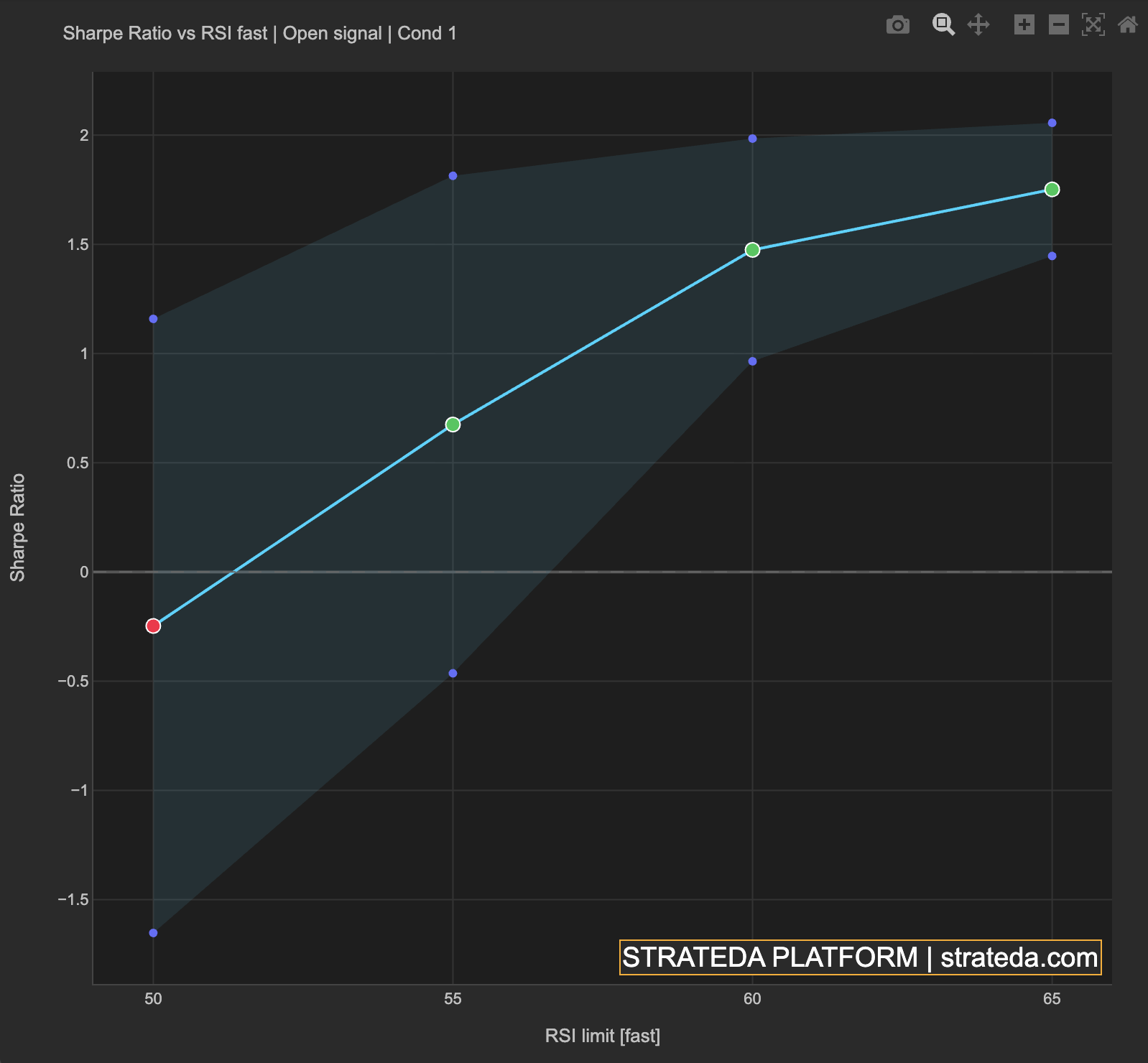
Figure 9: Sharpe ratio vs RSI limit value, sensitivity across four tested values
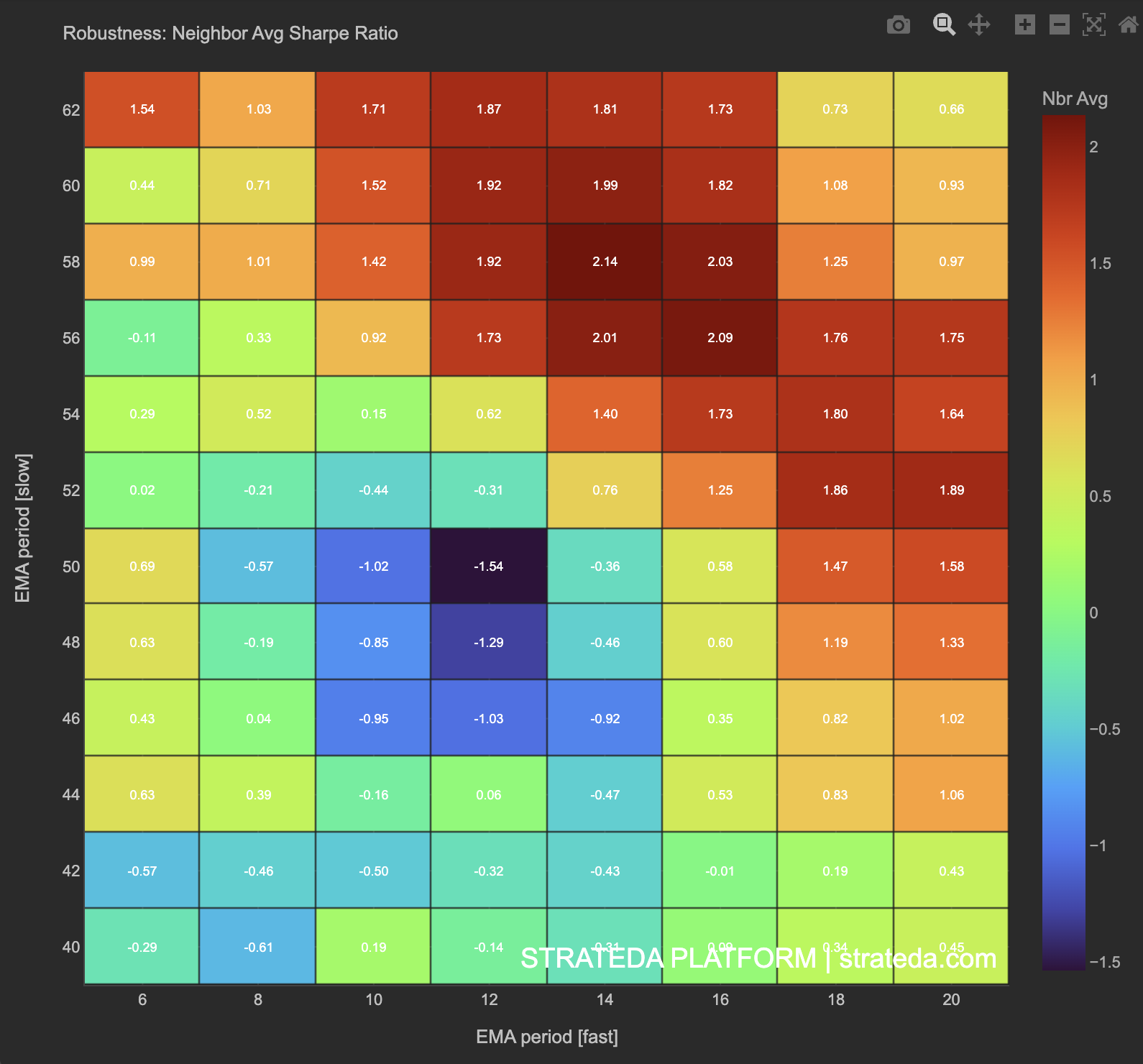
Figure 10: Robustness heatmap, neighbor-averaged Sharpe with RSI filter applied
Description of Results
The RSI sensitivity chart shows Sharpe improving consistently as the limit increases from 50 to 65. At limit 50, the median Sharpe is negative, indicating the filter is too restrictive and eliminates too many valid entry opportunities. At limit 55, the median improves but the distribution band remains wide. At limit 60, the median rises to approximately 1.48 with a tighter band. At limit 65, the median reaches approximately 1.75 with the tightest band of all four values.
The robustness heatmap shows the neighbor-averaged Sharpe across all RSI limit combinations tested simultaneously. A hot zone at fast EMA 12 to 16 combined with slow EMA 56 to 62 consistently outperforms the rest of the grid regardless of which RSI limit value is active, with the peak neighbor-averaged Sharpe reaching 2.14 at fast 14, slow 58. This means the EMA hot zone is robust not only to parameter perturbation within the EMA space but also to variation in the RSI limit value. Fast EMA values below 10 show negative neighbor-averaged Sharpe across all RSI values, confirming that very short fast periods are structurally unsuitable regardless of filter setting.
Interpretation
RSI limit 60 was selected despite limit 65 producing a higher median Sharpe. The sensitivity chart shows that Sharpe improves continuously with higher RSI limits, meaning looser filters generally produce better in-sample results. However, higher RSI limits allow entries during more advanced momentum conditions where the remaining upside is structurally smaller. Capping at 60 preserves entries that occur while momentum is still developing, which is the condition the strategy is designed to exploit. This is a forward-looking decision rather than a purely statistical one derived from the chart.
The robustness heatmap confirms that the EMA hot zone at fast 12 to 16 and slow 56 to 62 is a genuine structural feature of the parameter space and not an artifact of any single RSI limit choice. The region performs consistently well across all RSI values tested, which is stronger evidence of robustness than a region that only appears at one specific RSI setting.
Conclusion
The optimization and robustness analysis identified a confirmed hot zone at fast EMA 12 to 16 and slow EMA 56 to 62, consistent across all RSI limit values tested, with RSI limit 60 selected for the reasons described above. Rather than restricting the following WFO search space to this exact peak, the parameter ranges are kept the same, fast EMA 6 to 20 and slow EMA 40 to 62, to enable flexibility across changing market conditions. Each IS window will re-optimize independently within these ranges on its own training data, without knowledge of the following OOS period.
4. Walk-Forward Validation, 5 Windows
Method
Walk-forward optimization divides the data into rolling windows, each consisting of an in-sample training period followed by an out-of-sample testing period. The optimizer finds the best parameters on the training data, then tests those parameters on the out-of-sample period without further adjustment. This process rolls forward through the full data range, generating a series of independent out-of-sample results that collectively form a forward-tested equity curve.
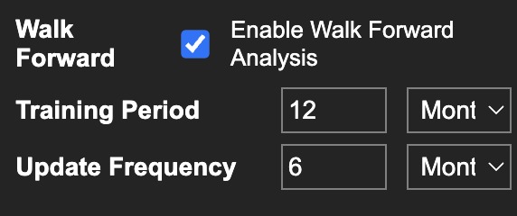
Figure 11: WFO configuration panel showing Walk Forward enabled, Training Period 12 months, Update Frequency 6 months
The configuration for the primary validation run is as follows. The training period is 12 months. The update frequency, which defines the out-of-sample window length, is 6 months. The data range spans January 2024 to March 2026, generating 5 rolling windows. The parameter search ranges for each IS optimization are those confirmed in the previous chapter, fast EMA 6 to 20, slow EMA 40 to 62, RSI(14) below 60. Each IS window re-optimizes independently within these ranges, selecting the best parameters for its specific period without knowledge of what follows.
The 12-month IS to 6-month OOS ratio of 2:1 is aligned with the recommended ratio for M30 strategies documented in Strateda's WFO window sizing guidelines, where market microstructure changes fast enough that older IS data has diminishing relevance for forward parameter selection.
Results
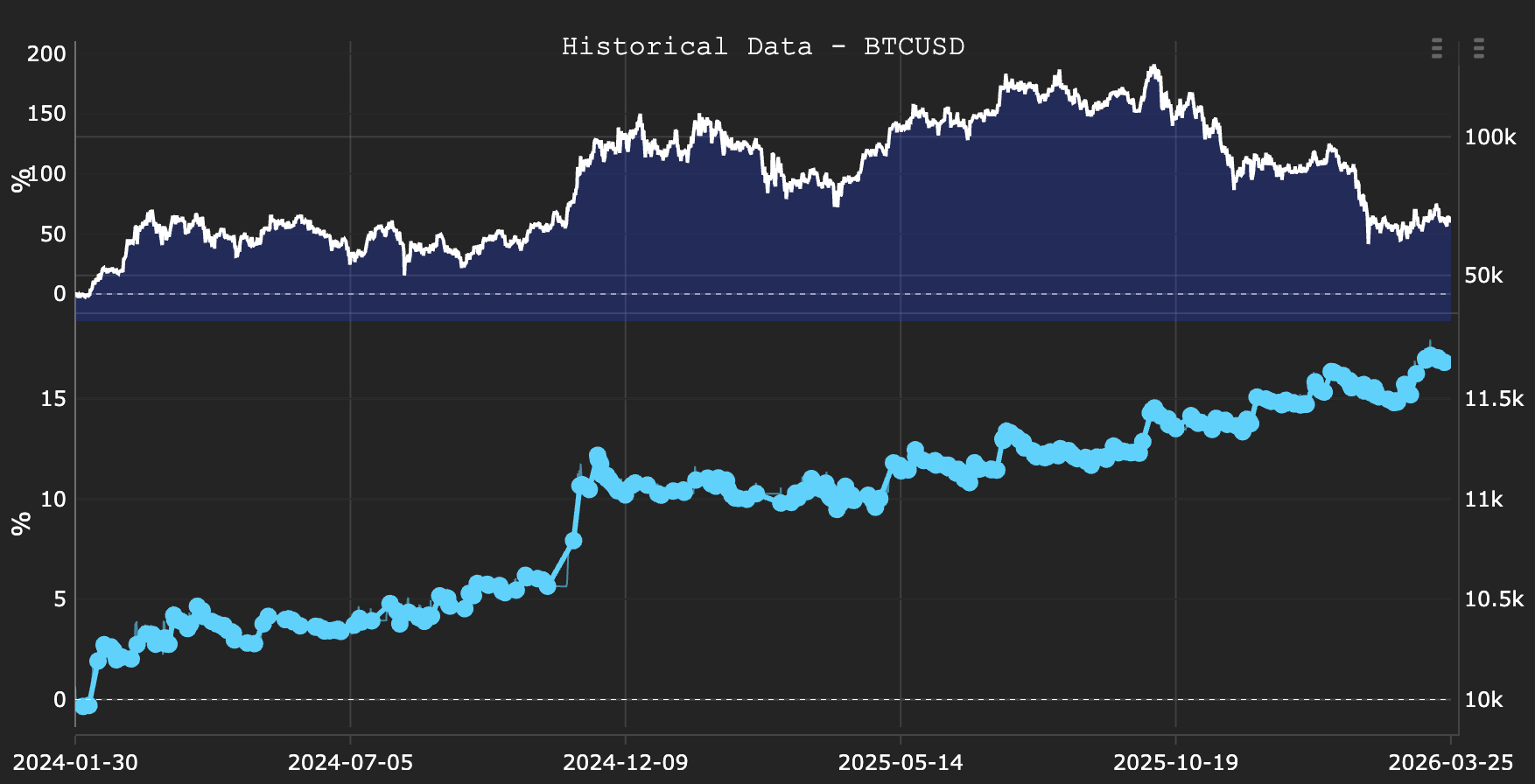
Figure 12: Combined OOS equity curve loaded in View Panel after WFO completes
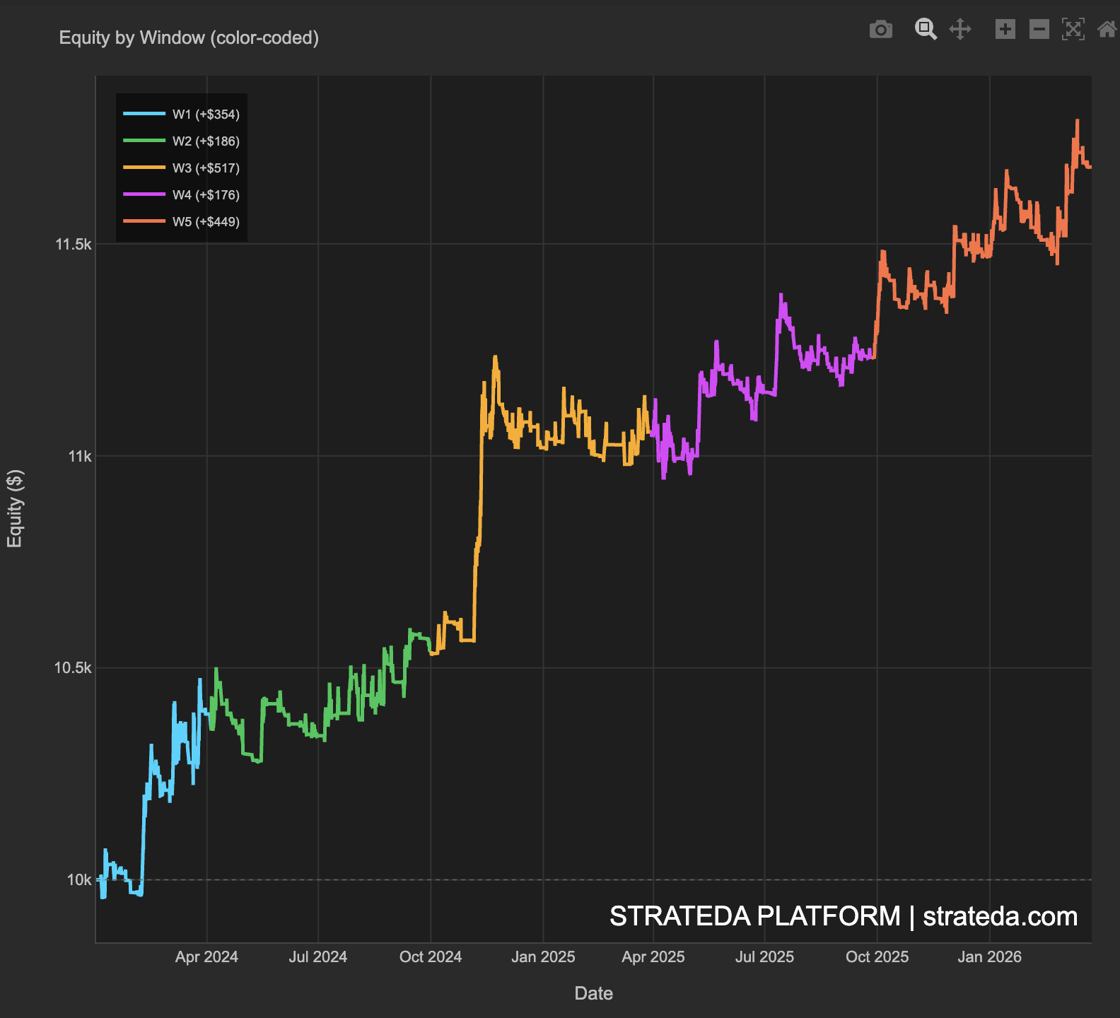
Figure 13: Equity by Window color-coded showing 5 windows January 2024 to March 2026
Description of Results
The combined OOS equity curve trends upward continuously from start to finish, built entirely from out-of-sample data across 5 independent windows. Every window produces a positive return, and the cumulative line shows no extended flat or declining phases.
Per-window out-of-sample returns are as follows. W1 produced 3.5%, W2 produced 1.9%, W3 produced 5.2%, W4 produced 1.8%, and W5 produced 4.5%. The cumulative OOS return across all 5 windows is approximately 17%. The average return per window is 3.36% with a standard deviation of 1.37%.
The IS versus OOS Sharpe chart shows IS Sharpe ranging from approximately 2.2 to 3.1 across windows, while OOS Sharpe ranges from approximately 0.97 to 2.78. A consistent degradation from IS to OOS is present in 4, but OOS Sharpe remains meaningfully positive throughout. In window 5 Sharpe of OOS slightly exceeds IS.
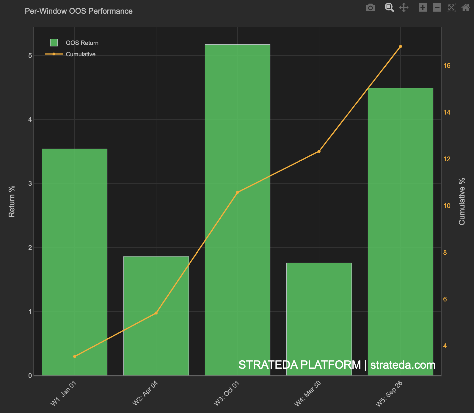
Figure 14: Per-Window OOS Performance, 5 windows with cumulative line
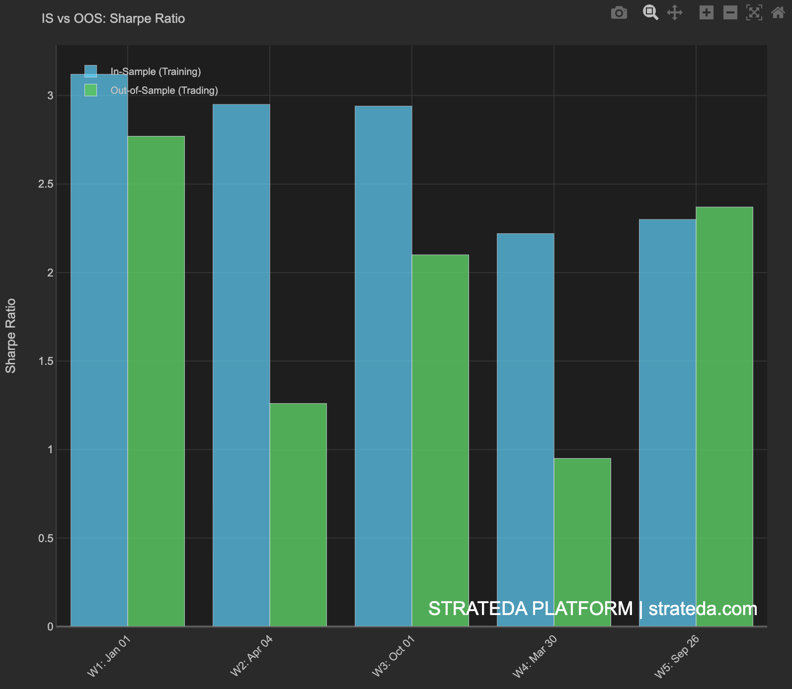
Figure 15: IS vs OOS Sharpe Ratio per window, 5-window run
The parameter stability chart shows the slow EMA holding (green) at 40 for W1 through W3, then shifting to 52 for W4 and W5. The fast EMA (blue) moves from 16 to 14 across the early windows, then drops to 6 for the two later windows. The parameter stability score is 0.74, just below the 0.75 threshold for high-stability classification.
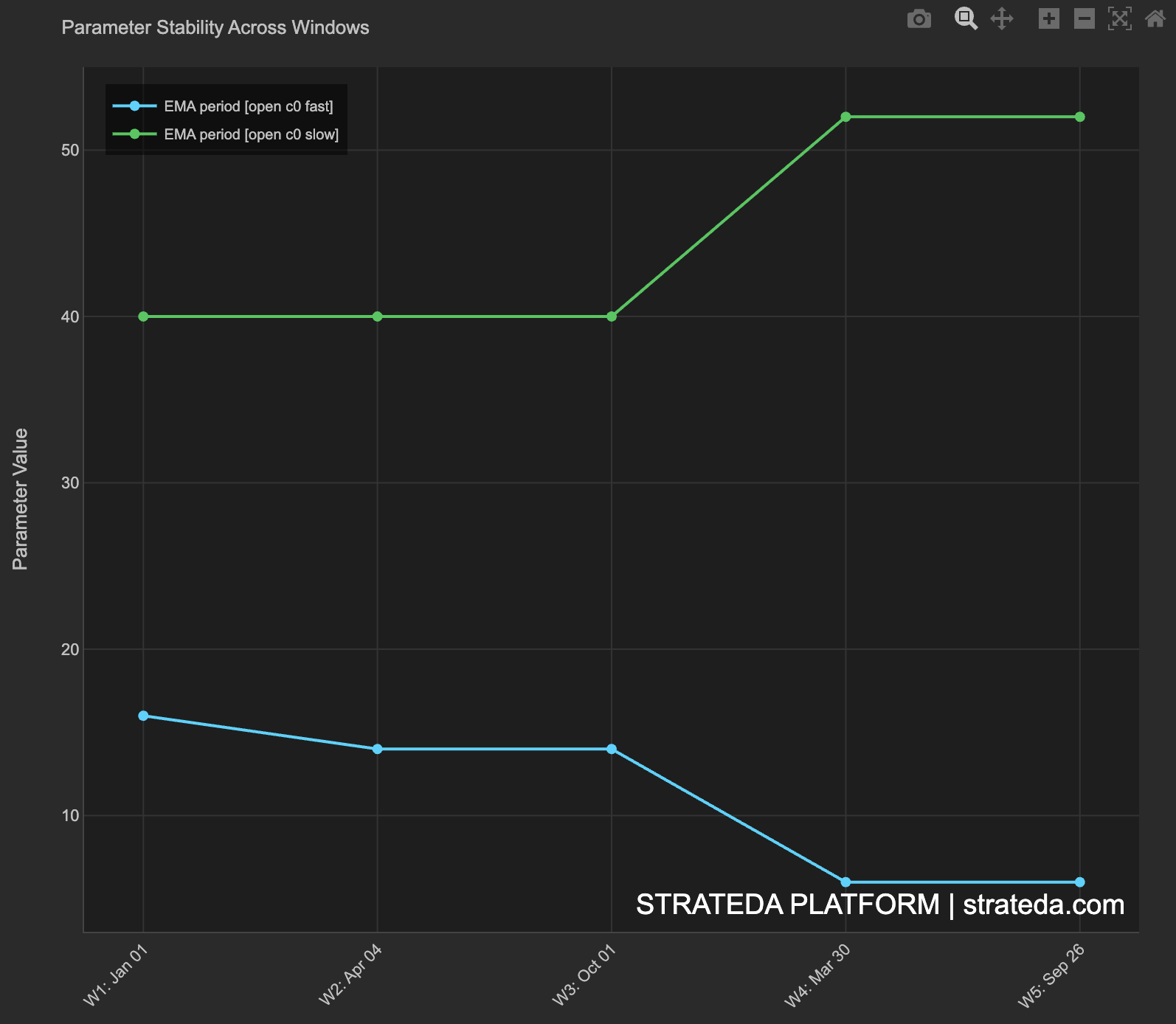
Figure 16: Parameter Stability across 5 windows, fast and slow EMA values
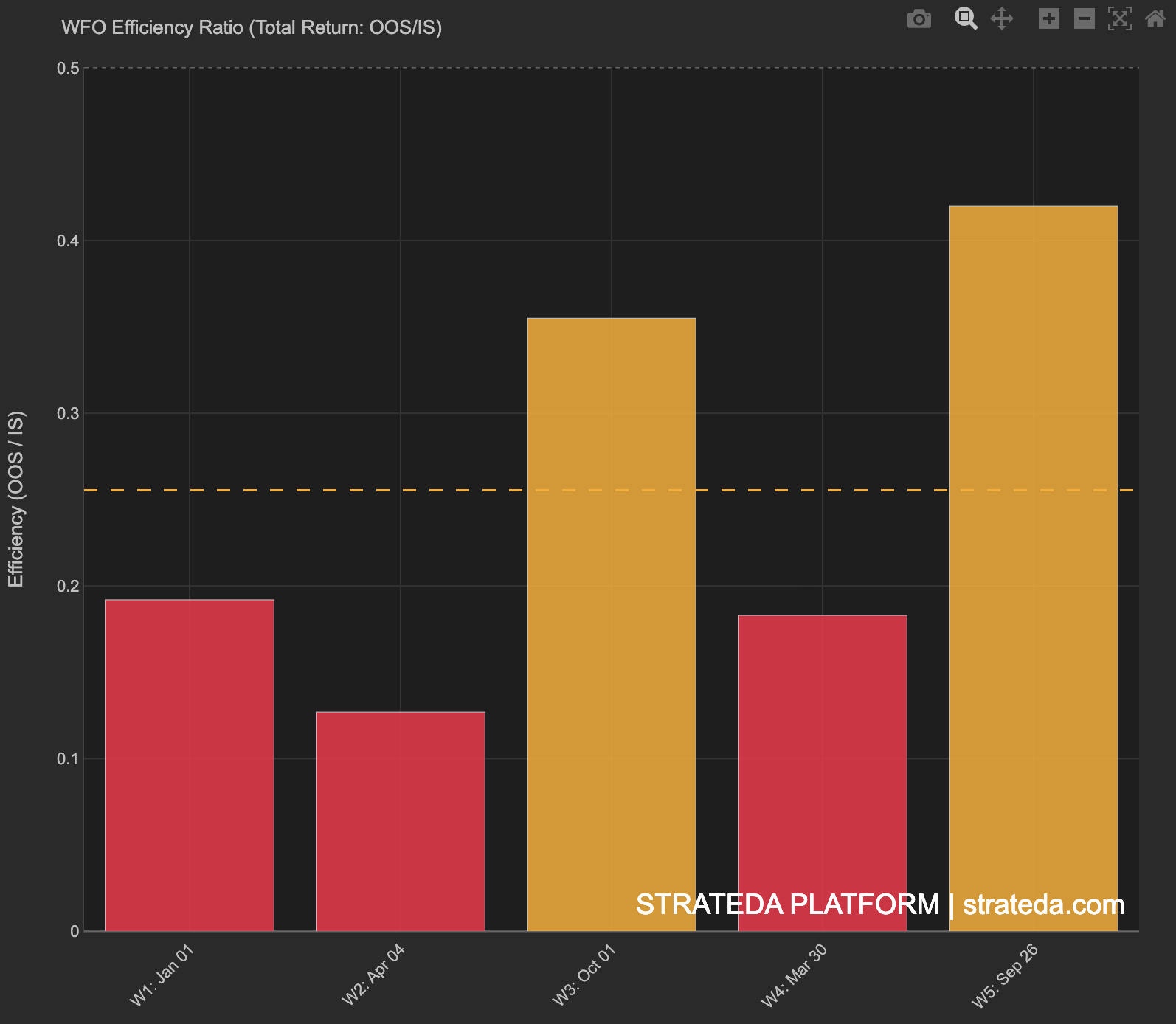
Figure 17: WFO Efficiency Ratio per window, all positive
The efficiency ratio bars are all positive, with W3 reaching approximately 0.35 and W5 reaching approximately 0.42. The Walk-Forward Factor average is 0.25.
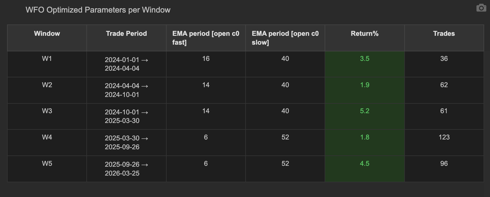
Figure 18: WFO Optimized Parameters per Window table for 5-window run
Interpretation
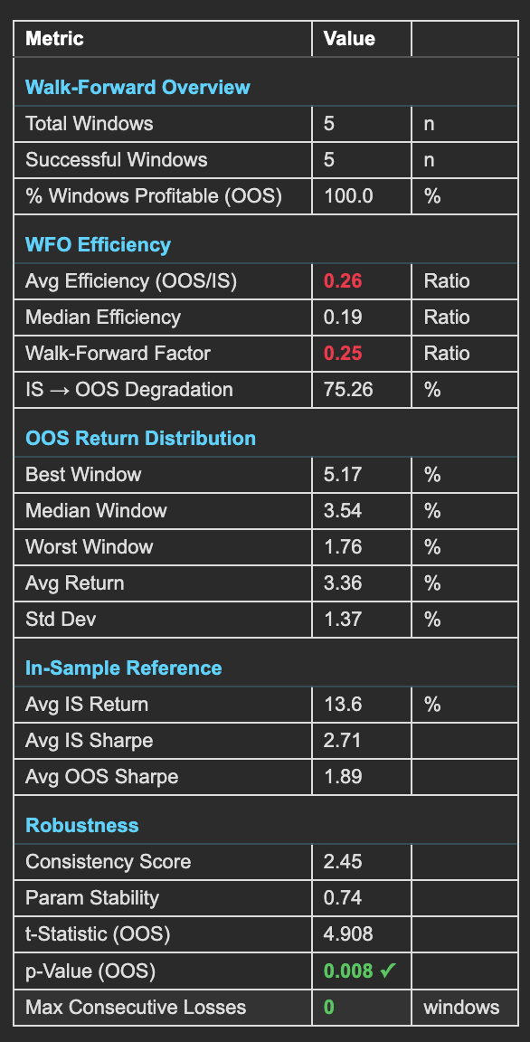
Figure 19: WFO Summary Statistics table for 5-window run
The p-value of 0.008 is the most significant number in this table. It is derived from the t-statistic of 4.908, computed from the mean OOS return of 3.36%, the standard deviation of 1.37%, and the window count of 5. The result falls well below the standard 0.05 significance threshold, indicating that the probability of observing five consecutive profitable windows by chance, given the variance in results, is less than 1%. This is statistical evidence that the OOS profitability is not a random outcome.
The Walk-Forward Factor of 0.25 and the IS to OOS degradation of 75.26% indicate that a significant portion of the IS performance does not carry through to OOS. This is expected behavior in any walk-forward analysis: the IS windows optimize on data they can see, and some portion of that performance reflects fitting rather than genuine forward signal. The critical question is whether OOS absolute performance is positive and consistent. In this run, it is. The Walk-Forward Factor being below the 0.3 threshold is a caution flag, but it does not override a p-value of 0.008 and 100% profitable windows. The low factor reflects the high IS Sharpe of 2.71 more than it reflects poor OOS performance.
The parameter stability score of 0.74, just below the 0.75 threshold, warrants monitoring. The shift in the optimizer selecting fast EMA values of 6 in W4 and W5, compared to 14 to 16 in the earlier windows, may indicate that the market has begun rewarding faster momentum signals in the 2025 to 2026 period. This is an observable early signal of potential parameter drift rather than a current concern.
The most significant individual finding is that W4 and W5 cover the period from March 2025 to March 2026. An examination of the BTCUSD price chart for this period shows that BTC was not in a clean uptrend. Price peaked in early 2025 and declined through much of the remainder of 2025 and into early 2026. A strategy that simply tracked BTC's directional movement would have produced negative returns during this period. The strategy returned 1.8% and 4.5% in these two windows, on data entirely outside the optimization year, during a period when holding a long BTC exposure was not inherently profitable. This is the most direct evidence that the crossover logic is capturing a real pattern rather than only riding a directional bull market.
Conclusion
The 5-window walk-forward validation produces a statistically significant result, 100% profitable out-of-sample windows, an average OOS Sharpe of 1.89, and a p-value of 0.008. The strategy demonstrates positive returns even during the declining BTC price period of 2025 to 2026, which was entirely unseen during the optimization phase. The evidence supports the hypothesis that a real edge exists in the current market regime. Five windows covering 2.4 years of data in a single regime is a strong result, but it leaves open the question of whether this regime has always existed or is a recent phenomenon. Chapter 5 addresses that question.
5. Regime Analysis, 11 Windows
Method
The 5-window run covers only the post-2024 market period. To understand whether the strategy has a genuine regime dependency and when the current regime began, the data range is extended back to March 2021, producing 11 rolling windows with the same 12-month IS and 6-month OOS configuration. This span covers BTC's 2021 bull top, the full 2022 bear market, the 2023 recovery period, and the 2024 to 2026 bull phase, providing the broadest possible regime diversity available within the dataset.
Eleven windows sits above the practitioner-grade threshold of 7 to 10 windows described in Strateda's window count documentation, providing sufficient statistical power to characterize regime behavior with confidence.
Results
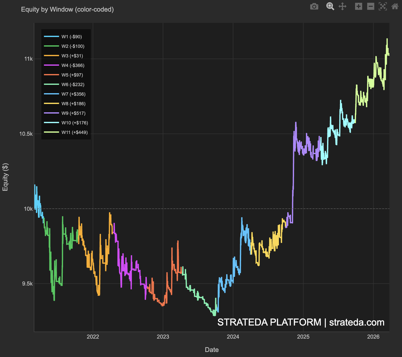
Figure 20: Equity by Window color-coded showing 11 windows March 2021 to March 2026
Description of Results
The equity by window chart shows a markedly different picture from the 5-window run. The combined equity curve falls from $10,000 through 2022, reaches a low near $9,300 in mid-2023, then recovers strongly through 2024 and 2025 to end near $10,900. The overall gain across the full 5-year period is approximately 9%, but the path is sharply non-linear, with clear phases of loss and recovery.
The per-window chart shows W1 through W6 as predominantly red bars, with W4 at -3.7% being the worst single window. W7 through W11 are entirely green, with W9 at +5.2% being the strongest. The cumulative line falls steadily through the first six windows, then rises consistently through the final five.
The efficiency ratio chart mirrors this pattern. W1 through W6 show red or near-zero bars. W7 through W11 show consistent positive bars above zero.
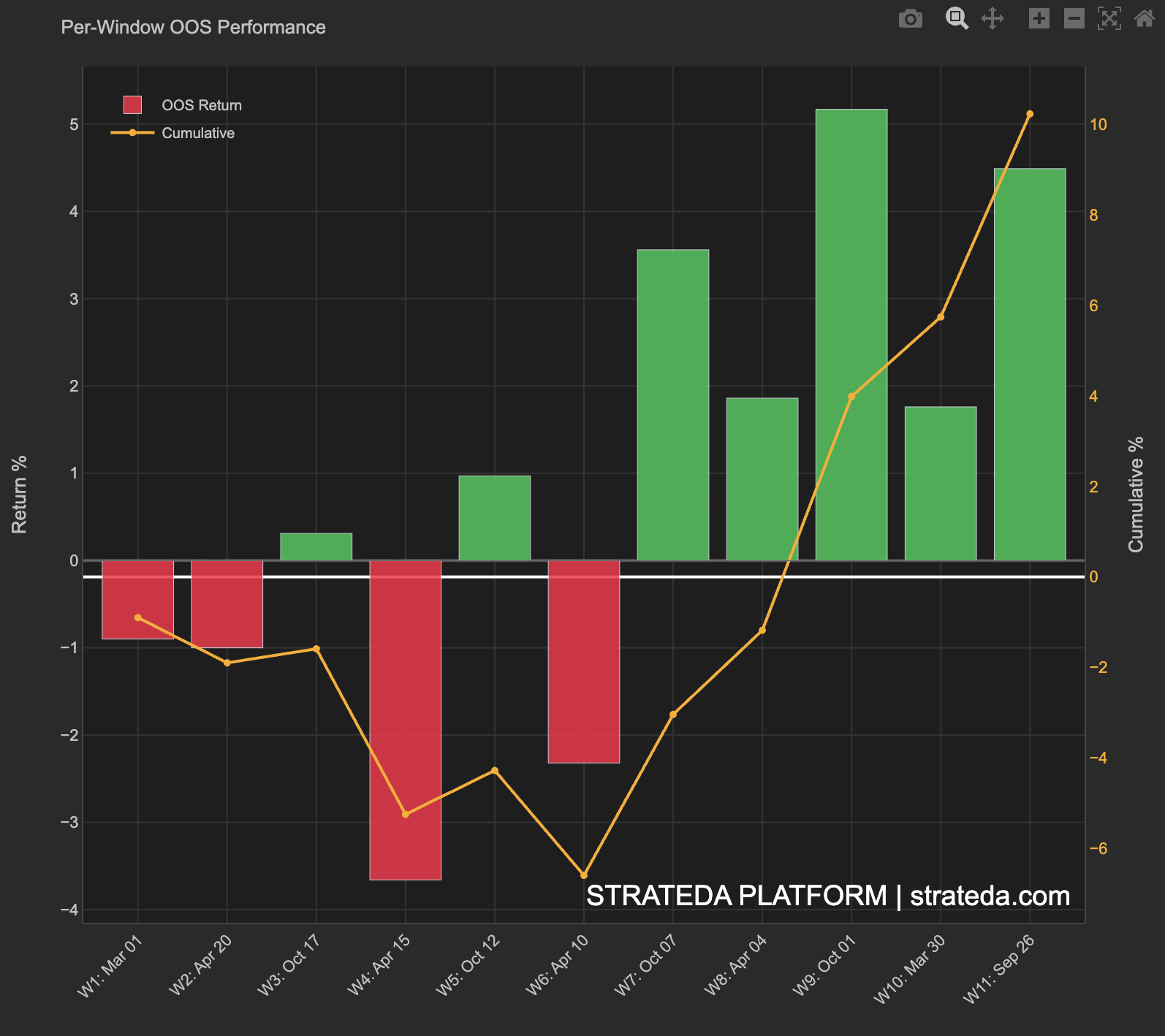
Figure 21: Per-Window OOS Performance, 11 windows with cumulative line
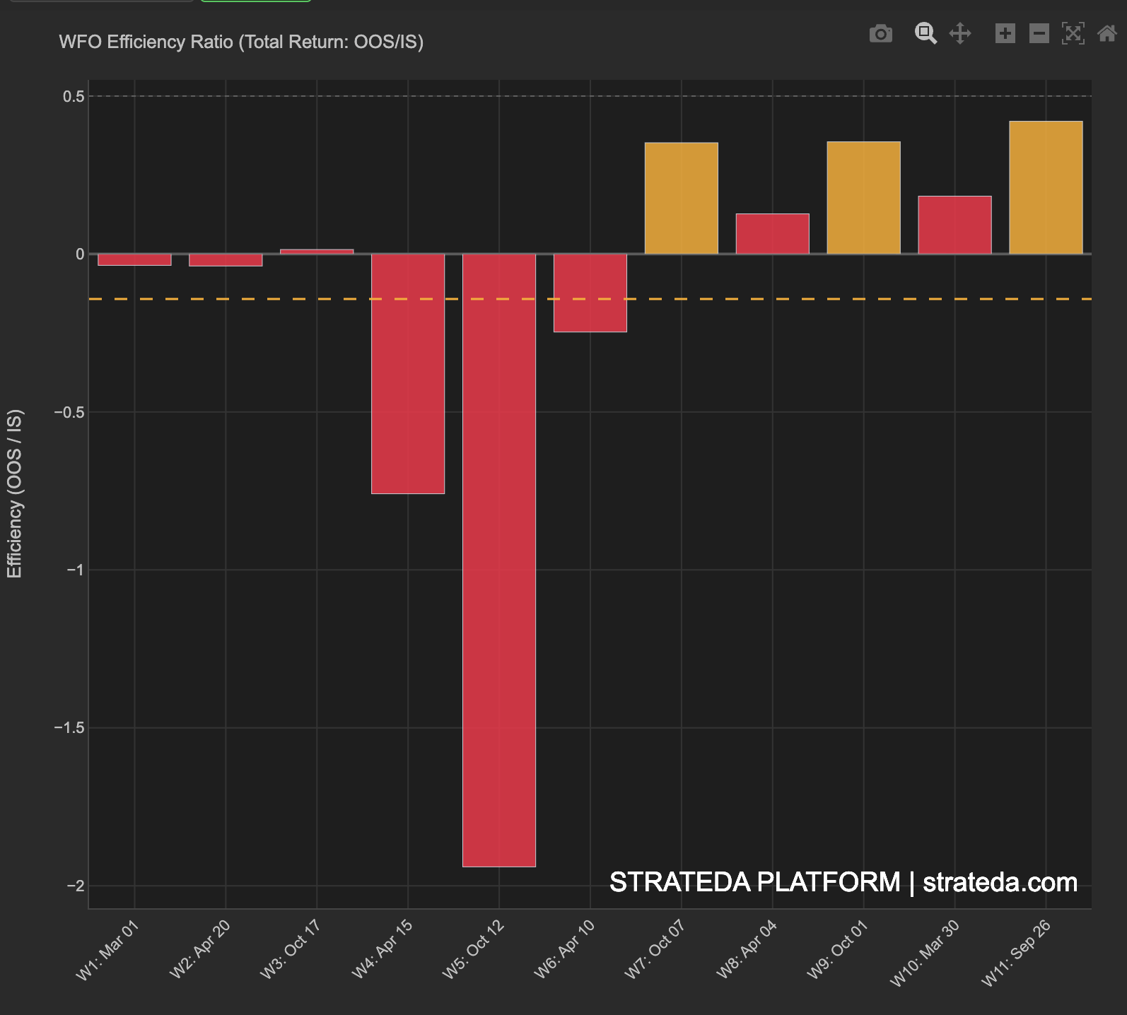
Figure 22: WFO Efficiency Ratio per window for 11-window run
The IS versus OOS Sharpe chart shows that during W1 through W6, IS Sharpe values are broadly positive, ranging from near zero to approximately 3.7, but OOS Sharpe values are mostly negative, reaching as low as approximately -4.1 in W6. From W7 onwards, both IS and OOS Sharpe are positive and the gap between them narrows substantially compared to the early windows.
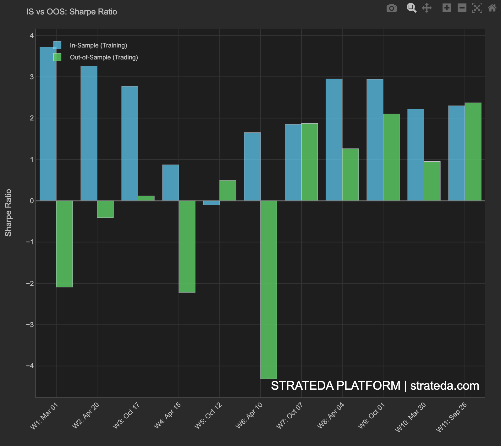
Figure 23: IS vs OOS Sharpe Ratio per window, 11-window run
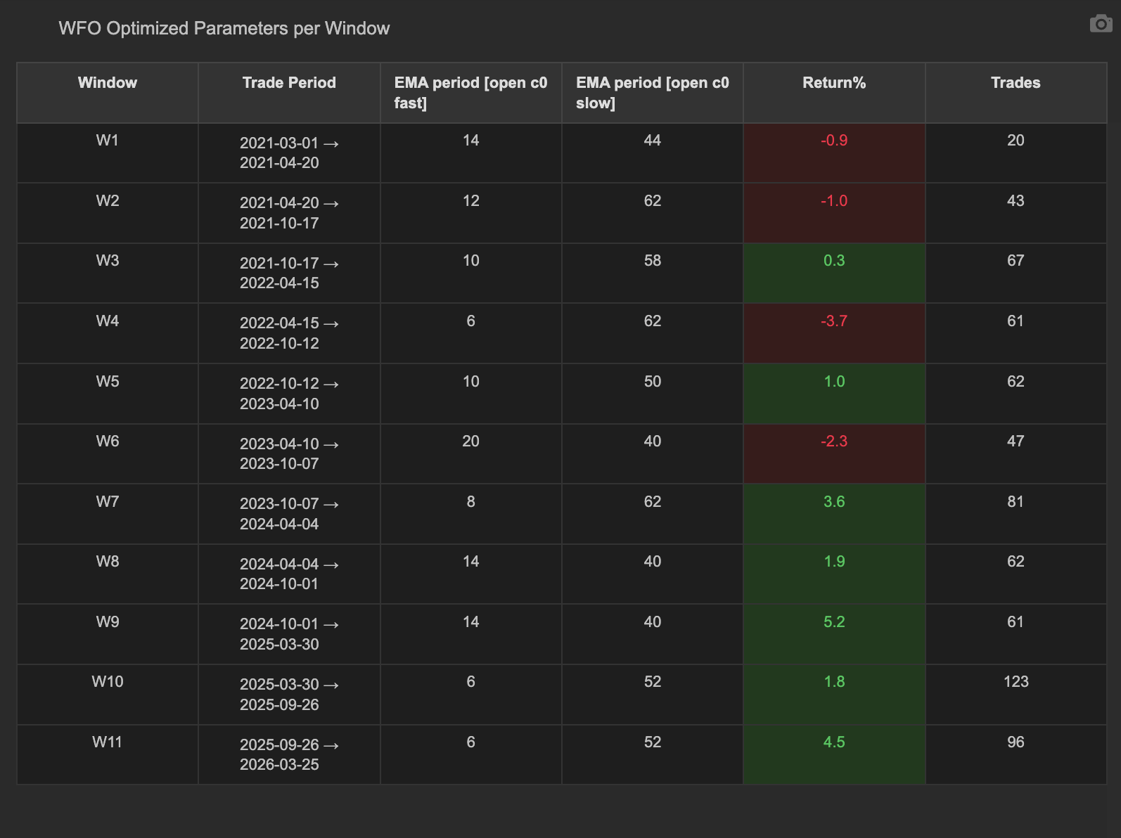
Figure 24: WFO Optimized Parameters per Window table for 11-window run
Interpretation
The regime boundary at late 2023 is the central finding of this analysis. The transition occurs at W7, covering the OOS period from October 2023 to April 2024. Before this point, the strategy consistently fails to generalize from IS to OOS. After this point, it consistently succeeds.
The parameter table provides a critical insight into the mechanism. W4, the worst performing window at -3.7%, selected parameters in the fast 6 and slow 62 range. W7, the first consistently profitable window, selected parameters in the fast 8 and slow 62 range. The parameter choices are not dramatically different between the losing and winning phases. The same optimizer, given the same search ranges, finds broadly similar-looking answers in IS data across both regimes. The difference in OOS performance is not driven by the optimizer selecting wrong parameters in the losing phase. It is driven by the forward market conditions being structurally different from the training conditions in those windows.
This distinction is important for interpreting what walk-forward optimization reveals. If the optimizer had selected obviously bad parameters during 2021 to 2023 and good ones during 2024 onwards, one might argue the IS window configuration needs adjustment. But the IS Sharpe values across W1 to W6 are positive, often strongly so. The optimizer is performing correctly each time. It finds the best parameters for each IS period, and those parameters then fail OOS because the market dynamic in the OOS period does not match the dynamic that was present during the training period.
This is the observable behavior of a momentum strategy operating across a regime change. The strategy logic captures directional momentum in trending markets. From 2021 through mid-2023, BTC was not in a sustained trending regime. It peaked and reversed from an all-time high, experienced a deep bear market driven by structural events in the crypto ecosystem, and then ranged in recovery patterns that consistently invalidated the momentum signals that had worked in each preceding IS period. From late 2023 onwards, BTC entered a phase of sustained directional movement, and the momentum signals began generalizing across windows consistently.
We observe this transition clearly in the WFO data. We cannot explain with certainty what structural change in the market caused it. The hypothesis carried forward is that the transition reflects a shift from a ranging and declining regime to a trending regime. The WFO data provides empirical support for when that shift occurred and how it affects strategy performance. This is what a neutral scientific analysis of a non-stationary dynamic system produces, observable patterns, measurable transitions, and probabilistic hypotheses, rather than causal explanations.
Conclusion
The 11-window analysis reveals a strategy with a clear and observable regime dependency. The strategy does not generalize in choppy, ranging, or declining BTC markets, as evidenced by five losing windows across 2021 to 2023. It generalizes consistently in trending BTC markets, as evidenced by five consecutive profitable windows from late 2023 to March 2026. The inflection point at W7 is a factual observation from the data. The 5-window validation from Chapter 4, which produced a p-value of 0.008 and 100% profitable windows, applies specifically to the post-W7 regime. Taken together, the two runs provide a complete characterization of the strategy, statistically significant in the current regime, with a documented history of failure in a prior regime that ended approximately 18 months before the most recent data point.
6. Monte Carlo Risk Framework
Method
The Monte Carlo analysis takes the actual trade outcomes from the validated strategy and reshuffles them randomly across 1,000 simulations, generating a distribution of possible equity paths and maximum drawdown outcomes. This quantifies how much of the equity curve's performance depends on the specific order in which trades occurred, and establishes the realistic range of drawdown outcomes under different trade sequences.
The analysis is performed on the refined strategy with the RSI(14) below 60 filter applied. This version produces 378 trades over the January 2024 to March 2026 period, compared to 682 trades in the baseline from Chapter 1. The RSI filter reduces trade frequency but improves signal quality, producing a total return of 16.81% and a Sharpe ratio of 1.92. The Monte Carlo framework uses these 378 actual trade outcomes as its input, making no assumptions about the distribution of returns. The simulations derive entirely from the empirical trade data.
The risk boundaries established in this chapter define when a live-running version of this strategy should be considered to be operating outside its validated envelope. Rather than using arbitrary drawdown thresholds, these boundaries are derived directly from the distribution of outcomes produced by the actual validated trade data.
Results
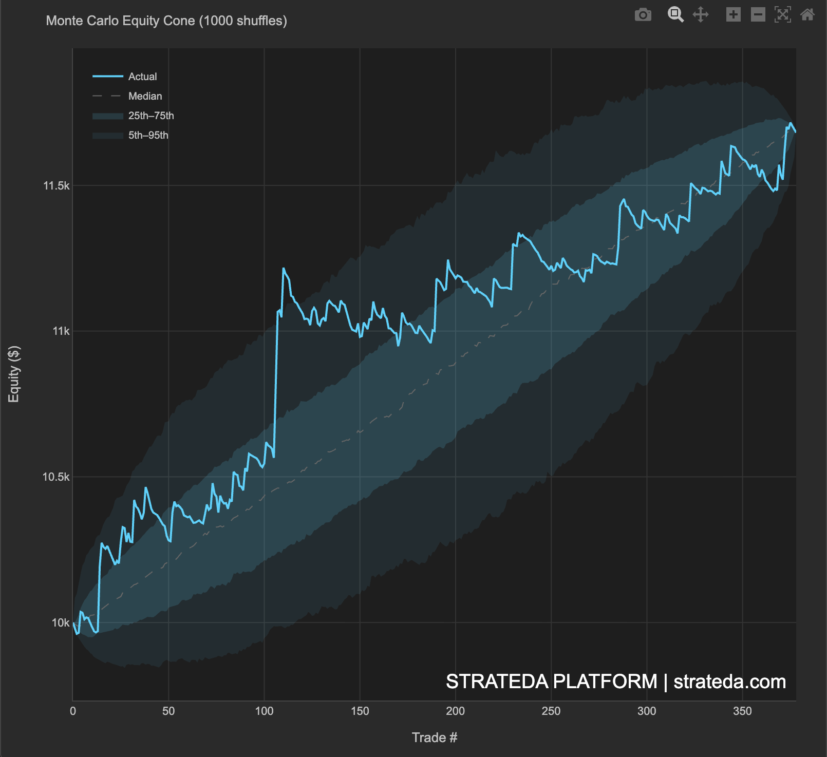
Figure 25: Monte Carlo Equity Cone showing actual equity curve against 1000 simulated paths with percentile bands
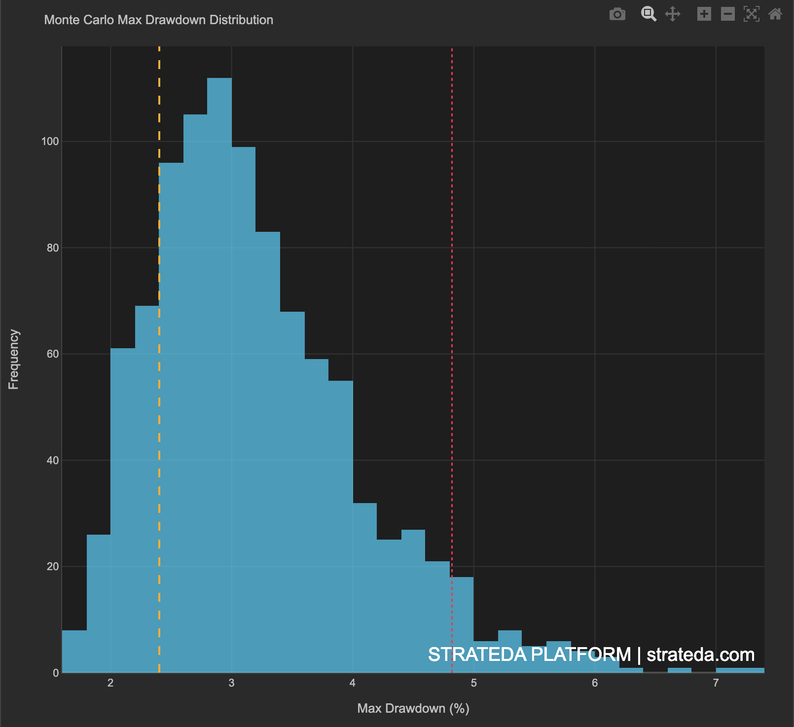
Figure 26: Monte Carlo Max Drawdown Distribution histogram with actual and 95th percentile reference lines
Description of Results
The Monte Carlo equity cone shows the actual equity curve in cyan, tracking above the median simulation line throughout the full period and remaining within the 25th to 75th percentile band. The outer band, representing the 5th to 95th percentile of all 1,000 simulations, shows that even in the worst 5% of simulated trade sequences, the strategy ends the period in positive territory.
The drawdown distribution histogram shows the median maximum drawdown across 1,000 simulations at approximately 2.9%. The actual observed maximum drawdown, marked by the orange line, is 2.4%. The 95th percentile maximum drawdown, marked by the red line, is 4.82%. No simulation out of 1,000 produced a maximum drawdown exceeding 10%.
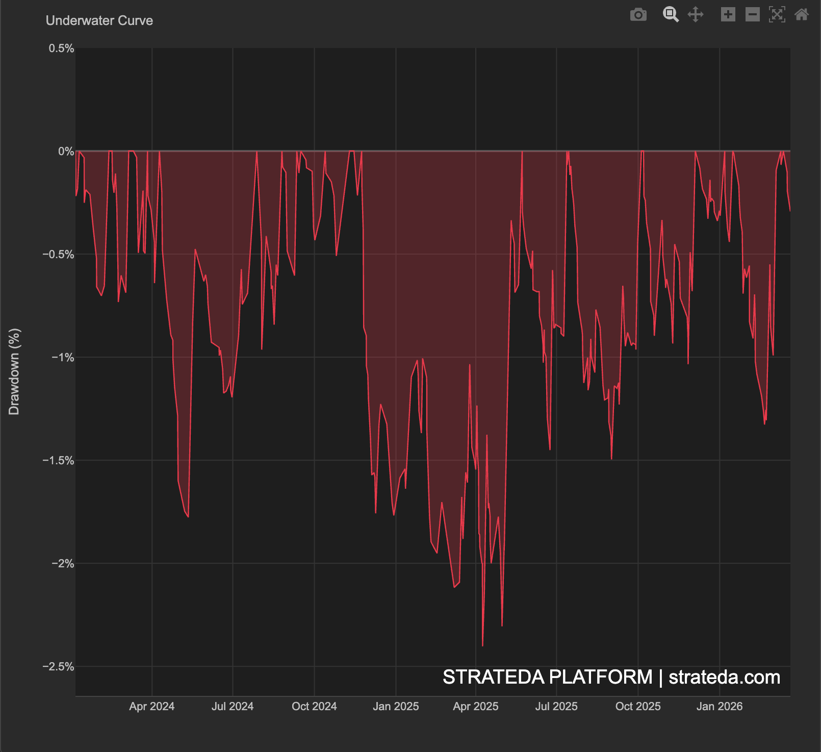
Figure 27: Underwater Curve showing drawdown depth and duration from January 2024 to March 2026
The underwater curve shows that across the full 2.4-year period, drawdowns never exceeded -2.5% and recovered consistently. The maximum drawdown duration was 180 calendar days, with depth remaining shallow throughout.
Interpretation
The position of the actual equity curve within the upper half of the Monte Carlo cone is a positive signal. It indicates that the actual trade sequence was somewhat favorable compared to a random ordering, but not unusually so. The curve does not depend on a fortunate clustering of large wins at the beginning to establish a high starting equity. The edge is distributed across trades rather than concentrated in a few exceptional outcomes.
The 95th percentile maximum drawdown of 4.82% is the primary risk planning number for this strategy. Under adverse but plausible trade sequencing, this is the realistic worst drawdown the strategy is expected to produce. At 20% margin sizing on a $10,000 account, a 4.82% drawdown represents a $482 decline from peak equity. A live drawdown exceeding this level would indicate the strategy is operating outside its validated risk envelope and would constitute a signal to pause and reassess whether the current regime remains consistent with the validated regime.
The zero probability of a 10% drawdown across 1,000 simulations confirms that catastrophic loss is not a realistic outcome at current sizing, provided the market regime remains consistent with the validation period. This is an important qualification, the Monte Carlo simulations reshuffle the actual trades from the current regime. They model sequencing risk within the current regime but do not model regime change. The stopping rule from the WFO analysis, one negative OOS window, remains the primary protection against regime change.
On position sizing, the strategy currently commits 20% of account balance per trade. The total return of 16.81% is measured against the full account balance. The Monte Carlo risk envelope defines exactly how far position sizing can be increased before the 95th percentile drawdown exceeds a chosen risk tolerance. Deriving the optimal position percentage from this distribution, rather than choosing it arbitrarily, is the subject of the next article in this series.
Conclusion
The Monte Carlo analysis confirms that the strategy's risk profile is well-characterized and predictable within the current regime. The 95th percentile maximum drawdown of 4.82% at current sizing provides a concrete, empirically derived risk boundary. The actual equity curve's position within the simulation distribution confirms that the OOS performance does not depend on a lucky trade sequence. The risk framework is complete, WFO provides the regime characterization and the stopping rule, Monte Carlo provides the intra-regime risk boundaries and the basis for position sizing optimization.
Conclusion
The central question of this report was whether an EMA crossover strategy on BTCUSD M30 has a genuine, repeatable edge or whether it simply captured the direction of a bull market. The analysis provides a clear answer, the strategy has a statistically significant edge in the current market regime, confirmed by a p-value of 0.008 across 5 independent out-of-sample windows, including two windows where BTC price was declining and a passive long exposure would have lost money.
The 11-window analysis adds the regime context that the 5-window result alone cannot provide. The strategy fails consistently from 2021 to mid-2023 and succeeds consistently from late 2023 onwards. The parameter choices across both phases are broadly similar. The performance difference is driven by market regime, not by optimization quality. This characterization is the most important output of the entire analysis, the strategy is a regime-specific tool, not a universal one.
The Monte Carlo analysis defines the operational risk boundaries. The 95th percentile maximum drawdown is 4.82% at current 20% margin sizing. A live drawdown exceeding this level, or one negative OOS window in a future WFO refresh cycle, are the observable signals that the strategy is operating outside its validated envelope.
A deployment hypothesis can be formulated as follows. Run the strategy in the current regime with parameters refreshed every 6 months via a new WFO cycle o updated data. The strategy is stopped when one OOS window produces a negative return, or when the IS to OOS efficiency ratio shows a sustained decline across consecutive windows, or when the OOS Sharpe drops below zero. Within the current regime, the Monte Carlo 95th percentile maximum drawdown of 4.82% serves as the intra-regime risk boundary. A live drawdown exceeding this level indicates the strategy is operating outside its validated envelope and requires an immediate pause and reassessment.
Run this analysis on your own strategy at Strateda
Walk-Forward Optimization is available on Premium plans. Parameter optimization with full analytics including heatmaps, robustness analysis, and equity curve fan is available on Plus plans and above. Monte Carlo simulation, underwater curve, and the full backtest analytics suite are included on Plus plans and above. Compare all plan features
This article is part of a research series on the complete strategy lifecycle.
You are here: Walk-Forward Optimization, validating whether a strategy's edge is real and characterizing the conditions in which it operates.
Next: Position Sizing and Capital Efficiency. Given a validated edge and a defined risk envelope, how aggressively should the strategy be deployed? The next article derives the optimal position size from the Monte Carlo risk distribution using the same BTCUSD strategy as the case study.
Following: Transaction Cost Analysis. Connecting WFO predicted returns to what live broker execution actually delivers, including slippage distributions, latency patterns, and execution precision on real trades.