Transaction Cost Analysis: What Live BTCUSD Execution Data Reveals About Real Trading Costs
Estimated reading time: 30 minutes
Introduction
Transaction cost analysis is the systematic measurement of the gap between the price a strategy intended and the price a broker delivered. It does not measure whether a strategy has an edge. That question is answered by backtesting and walk-forward validation. TCA answers a different question. Once a signal is generated and sent for execution, what do execution costs actually look like, and how large are they relative to the capital committed?
This question is almost never answered with real data. Traders build strategies, optimize them, validate them, and deploy them live. The execution layer is treated as a constant. Spreads are modelled with assumptions. Slippage is either ignored or set to a round number. The result is a systematic blind spot in the strategy development process. It is also a reliable source of the gap between backtest performance and live results.
This report fills that blind spot with direct measurement. Across nine days of live trading from April 1 to April 9, 2026, an EMA 2/5 crossover strategy on BTCUSD M1 generated 2,723 trade signals through a major CFD broker accessed via MetaTrader 5. Every fill was recorded. Every signal delivery timestamp was logged. The analysis covers signal delivery latency, slippage at entry and exit, temporal execution patterns, and the cost of slippage expressed as a percentage of margin committed per trade.
The strategy itself is not the subject of this report. An EMA 2/5 crossover on M1 is a high-frequency configuration that generates a large trade volume. It was chosen for that reason. The strategy is deliberately unprofitable over the analysis period. The signal quality is not the point. The point is the 1,336 completed fills it generated, which provide a statistically robust foundation for measuring execution quality. For strategy validation methodology, see the preceding article in this series.
The central finding is not complicated. At high leverage on a major CFD instrument, a nominal spread-driven slippage of 12 price units per entry translates to approximately 5.1% of broker margin per fill. That number is not directly readable from a broker's fee schedule or account documentation. An estimate is possible, but it requires knowing your effective leverage per trade, your typical spread, and your exact lot sizing after broker rounding constraints are applied. All three inputs carry uncertainty in practice. Direct measurement from live fills resolves that uncertainty. This report shows how to measure it, what the measurement reveals, and why it matters for any live deployment on a leveraged instrument.
The report is organized as follows. Chapter 1 defines slippage precisely and describes the measurement setup. Chapter 2 explains the signal delivery architecture. Chapter 3 examines signal delivery stability as a system property. Chapter 4 analyzes the slippage distribution and identifies what it actually represents. Chapter 5 examines slippage over time and across the trading week. Chapter 6 presents two independence findings. Chapter 7 identifies temporal execution patterns. Chapter 8 quantifies execution cost as a function of leverage and margin. The conclusion connects these findings to position sizing and live deployment.
1. Methodology and Definitions
What Slippage Measures
Slippage in this analysis is defined as the difference between the actual broker fill price and the theoretical target price at the moment the signal was generated. The theoretical target price is the last candle close price, the price on which the strategy's entry and exit conditions were evaluated when the signal fired.
This definition is precise and consequential. Slippage does not measure broker execution quality in isolation. It measures the combined effect of everything that happens between the candle closing and the fill confirming. This includes the time for Strateda's cloud server to evaluate the signal, the transmission delay from Strateda's server to the MT5 Expert Advisor, the time for the EA to route the order to the broker, and the broker's internal processing and execution. All of these components are captured in a single observable number, the difference between the signal price and the fill price.
This is the correct definition from a strategy perspective. Every systematic strategy must answer a single question. "If my signal fires on the close of this candle, what price do I actually receive?" The answer is the fill price. The gap between the two is the execution cost the strategy bears, regardless of where in the chain it originates.
Instrument and Strategy
The instrument is BTCUSD, traded as a CFD on a standard account through a major broker accessed via MetaTrader 5. A standard account means commission is embedded in the spread rather than charged separately. Every cost associated with entering or exiting a position is reflected in the fill price. There is no separate per-lot commission. The slippage measurements in this report therefore represent the all-in execution cost per fill.
The strategy is an EMA 2/5 crossover on M1 candles. It was selected for its high signal frequency, which provides a large sample within a short observation window. The strategy is not optimized or walk-forward validated. Its purpose here is to generate fills, not to demonstrate an edge. All trades were executed on a demo account. Demo accounts at this broker replicate live spread and margin conditions. Fill quality on a live account may differ, particularly during high-volatility moments.
The observation period is April 1 to April 9, 2026. Total signals generated were 2,723. Total completed round trips with both entry and exit recorded were approximately 1,318. The difference reflects trades still open at the time of analysis and a small number of signals without complete fill data.
Data Source
All data is sourced from the Strateda live trading execution log, which records every signal generation timestamp, fill price, fill timestamp, margin used, and account balance at execution time. Signal delivery latency is measured as the time from signal generation on Strateda's cloud server to reception by the MT5 EA. This is a direct measurement from the log, not an estimate.
2. The Signal Delivery Architecture
Before interpreting any data, the execution chain needs to be understood clearly. There are two distinct steps between a signal firing and a position opening.
Step 1: Signal delivery. Strateda's cloud server evaluates the strategy conditions on candle close and transmits the trade signal to the MT5 Expert Advisor running on the trader's terminal. The latency charts in this report measure this step.
Step 2: Broker execution. The MT5 EA receives the signal and routes the order to the broker. The broker processes and executes the order and returns a fill confirmation. This latency is not directly measured separately, but its effect is captured in the slippage measurement.
Slippage captures the total cost of both steps as a price difference. Latency measures only Step 1.

Figure 1: The two-step execution chain. Signal delivery latency covers the Strateda→MT5 segment. Broker execution latency covers the MT5→broker segment. Slippage measures the combined effect of both as the observed difference between the signal price and the fill price.
Both segments can be reduced by selecting the server region closest to the MT5 terminal. Strateda operates dual-region servers in US East and EU Central. A terminal running on a US East VPS with the US East region selected reduces signal delivery time directly, and as a secondary effect also reduces broker execution latency, since most broker infrastructure is located near US financial centers. The data in this report was collected on the EU server configuration. A US setup would show shorter signal delivery times. Whether these differences affect execution quality for this strategy type is addressed in Chapter 6.
3. System Stability: Signal Delivery Latency
Method
Signal delivery latency is measured for every trade signal across the nine-day observation period. Both entry (OPEN) and exit (CLOSE) signals are measured independently. The distribution characterizes the stability of the signal delivery pipeline as a system property.
Results
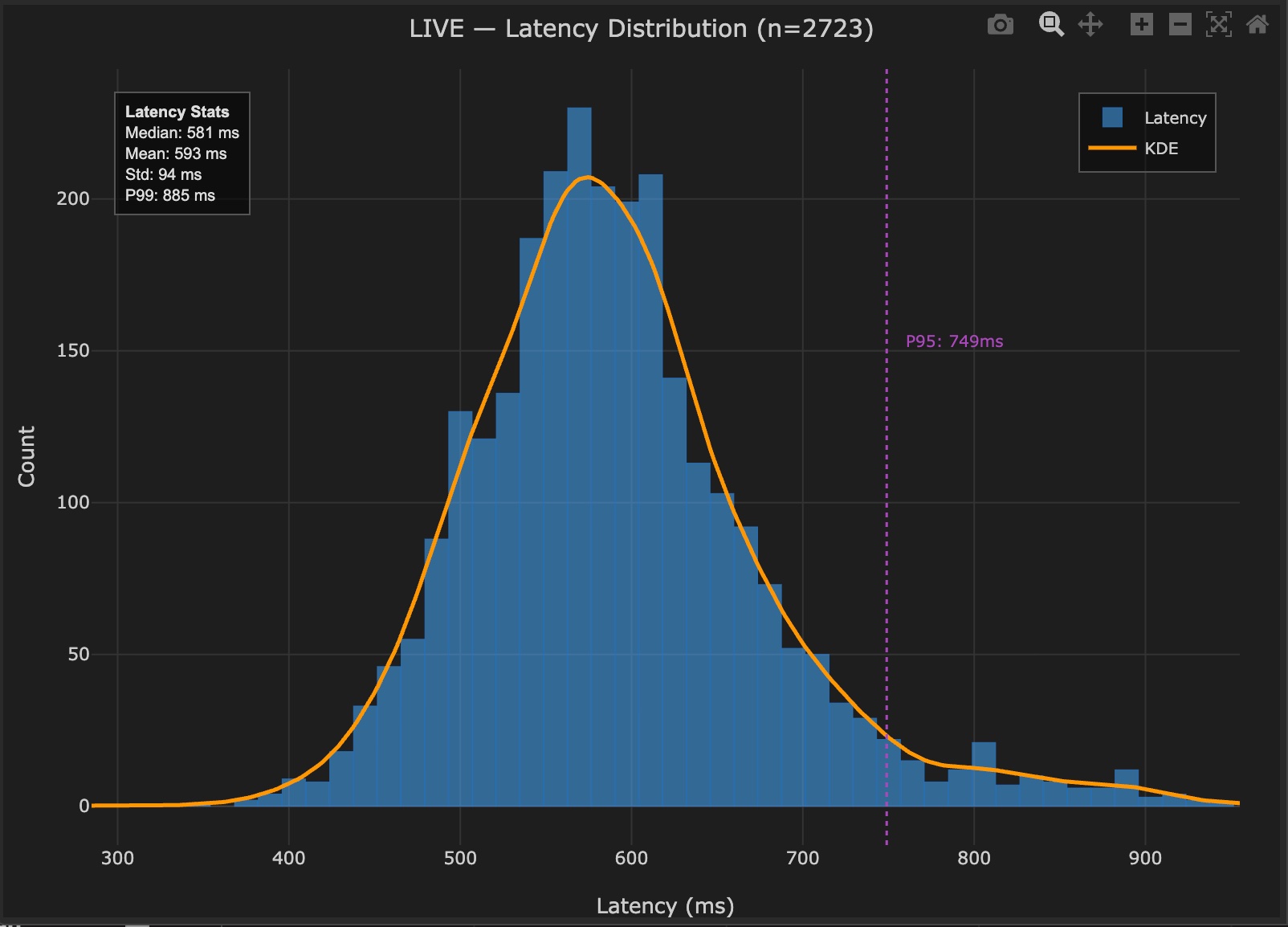
Figure 2: Signal delivery latency distribution, n=2,723. Median 581ms, mean 593ms, standard deviation 94ms, P95 749ms, P99 885ms.
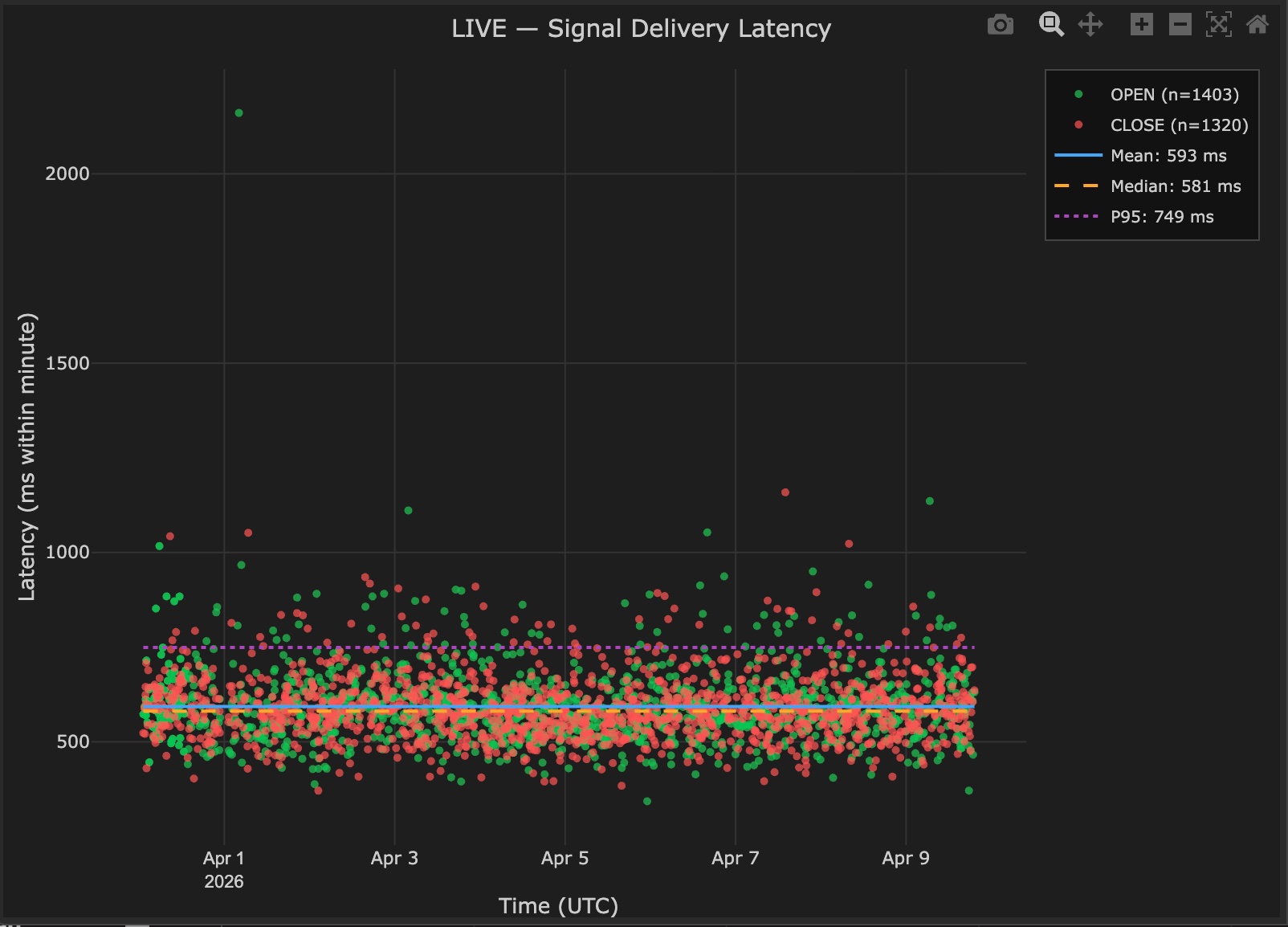
Figure 3: Signal delivery latency over time, April 1–9. OPEN signals (green, n=1,403) and CLOSE signals (red, n=1,320). The band is stable throughout with no visible drift or degradation.
Description of Results
The latency distribution is close to Gaussian. The median is 581ms, the mean is 593ms, and the standard deviation is 94ms, corresponding to a coefficient of variation of 16%. The P95 is 749ms and P99 is 885ms. The distribution spans approximately 300ms to 900ms, with a small right tail extending to isolated outliers. The shape indicates that the vast majority of signals are delivered within a narrow and predictable window.
The latency over time chart shows the full scatter of 2,723 signals across nine days. The band of points is stable throughout with no visible trend, no response to the sharp BTCUSD price movements that occurred during the period, and no systematic difference between OPEN and CLOSE delivery times.
Interpretation
The near-Gaussian shape is meaningful. A Gaussian distribution indicates a process dominated by random variation rather than systematic intermittent failures. If the delivery pipeline were unstable, subject to queuing delays, network congestion, or processing spikes, the distribution would show a heavier right tail or a bimodal structure. Neither is present.
The standard deviation of 94ms around a 581ms median represents approximately 16% variation. For an M1 strategy, where each candle represents 60 seconds, this variation is negligible. Even the P99 of 885ms represents delivery within the first 1.5% of the candle's lifetime. Signals are always delivered well within the candle window in which they were generated.
The stability over time confirms this is not an artifact of a particular period. The distribution observed on April 1 is consistent with April 9. System stability in practice is not the absence of variation. It is variation that is bounded, predictable, and independent of external conditions.
Conclusion
Signal delivery latency is stable, predictable, and well within acceptable bounds for M1 execution. The near-Gaussian shape with 94ms standard deviation characterizes this as a controlled system property. This chapter establishes the performance baseline for the signal delivery layer. The remaining chapters examine what happens after the signal arrives at the broker.
4. The Spread as Slippage: Entry and Exit Distribution
Method
Slippage is calculated for every entry and exit fill as the difference between the actual fill price and the last candle close price at signal generation time. For BUY entries, positive slippage means the fill occurred above the signal price. For close exits, negative slippage means the fill occurred below the signal price. Entry and exit distributions are analyzed separately.
Results

Figure 4: Slippage distribution for entries (green, n=1,336) and exits (red, n=1,321). Entry distribution: median 12.00, mean 12.10, std 11.73. Exit distribution: median 0, mean −0.349, std 10.97.
Description of Results
The two distributions tell fundamentally different stories.
The entry distribution is shifted entirely to the right of zero. The median is 12.00 price units, the mean is 12.10, and the standard deviation is 11.73. The distribution has a dominant peak at approximately 12 price units, a sharp, tall bar, with a tail extending to the right and almost no mass to the left of zero.
The exit distribution is centered at zero. The median is exactly 0, the mean is −0.349 price units, and the standard deviation is 10.97. The distribution is approximately symmetric around zero with a sharp spike at the center. There is no systematic shift in either direction.
Interpretation
The entry distribution is not measuring random execution noise. To understand what it does measure, the broker's quote and candle structure needs to be clear.
MT5 broker candles are constructed from the bid price stream. The candle close price is the last bid price before the candle closed. This is the signal price in this analysis. When a BUY order is placed, the broker fills it at the ask. The ask is always higher than the bid. The difference between ask and bid is the spread.
The fill price on a BUY entry therefore exceeds the signal price by approximately the full spread on every single trade. This is not slippage in the sense of poor execution. It is the structural cost of crossing the spread on a standard CFD account where commission is embedded in the spread rather than charged separately.
With 1,336 entries, this cost becomes directly readable in the histogram. The dominant bar at 12 price units is the spread. MT5 BTCUSD candles close at the bid. A BUY order fills at the ask. At approximately 12 price units for BTCUSD at this broker, that is exactly what the histogram shows. The scatter of fills around that peak reflects genuine price movement during the execution window. In the time between the candle closing and the fill confirming, the market moves, producing a distribution of outcomes above and below the spread level.
The exit distribution's centering at zero reveals the other side of this structure. When a long position is closed, a SELL order executes at the bid. The signal price is also bid-based. The reference and the fill are on the same side of the spread. The net result is that exit slippage averages near zero. Price movement during the execution window produces symmetric variation above and below zero with no structural cost in either direction. The mean of −0.349 confirms this. There is a marginal favorable bias on exits, not adverse.
This entry/exit asymmetry is a direct consequence of how MT5 bid-based candles interact with CFD standard account cost models. The spread is a one-way cost on entry. A BUY crosses from bid to ask. A SELL to close stays on the bid side. It is not a round-trip constant.
Conclusion
The slippage distribution at entry is centered at the spread, not at zero. The dominant bar at 12 price units is not noise. It is the broker's spread made directly readable by the volume of fills. The scatter around that peak is real market movement during the execution window. The exit distribution, centered at zero with a marginal favorable mean, confirms that the spread is paid at entry and not at exit. With 1,336 entries, this structure is statistically unambiguous. It is the most important single chart in this analysis.
5. Asymmetry Over Time and the Weekend Effect
Method
The per-trade slippage for entries and exits is plotted chronologically across the observation period. This view examines whether the entry/exit asymmetry is persistent across time and whether variation within the trading week is observable.
Results
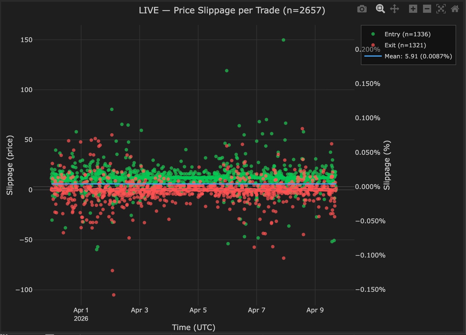
Figure 5: Price slippage per trade, April 1–9. Entries (green, n=1,336) form a persistent band above zero. Exits (red, n=1,321) are centered at zero. Mean combined slippage: 5.91 price units (0.0087%). Scatter dispersion visibly narrows over the April 3–6 weekend period.
Description of Results
The entry scatter forms a band persistently above zero throughout the full nine days. The band is centered around 10–15 price units with outliers extending upward to 50–150 price units. The exit scatter forms a symmetric band around zero with roughly equal mass above and below throughout the period.
The combined mean of 5.91 price units (0.0087% of price) reflects the blended average of entries centered near +12 and exits centered near 0. This is consistent with the distribution analysis in Chapter 4.
A visible change occurs over the weekend of April 3–6. The scatter of both entry and exit points narrows noticeably. The outliers above 50 price units disappear and the width of the main band compresses. This reverses when trading resumes Monday April 7.
Interpretation
The persistence of the entry band above zero across the full nine days confirms that the spread cost is not an artifact of any particular session, day, or volatility regime. It is a structural feature of every fill observed, present during periods of elevated BTCUSD price movement and periods of relative calm alike.
The weekend effect is a direct result of reduced market participation. On weekends, most major financial markets are closed. BTCUSD continues to trade, but with lower overall activity and more muted price movement. With less ambient price movement in the execution window, the dispersion of slippage around the central spread cost compresses. The central bar, the spread itself, does not change. What changes is the variability around it, because there is less price movement randomizing outcomes above and below the spread level.
This observation has a practical dimension for any 24/7 BTCUSD strategy. Weekend execution produces less slippage variance, not better execution per se. The spread cost remains. For strategies with signals that cluster around session openings or high-activity periods, this weekend pattern represents a structurally different execution environment that will appear in any temporal analysis of live data.
Conclusion
The entry/exit asymmetry from Chapter 4 is stable across the full observation period. The spread cost is present and constant in direction regardless of time of day, day of week, or market volatility level. The weekend effect demonstrates that the variance of slippage responds to market activity while the structural level does not. Both findings are consistent with a well-characterized execution environment.
6. Two Independence Findings
Method
Two specific relationships are tested that, if present, would indicate systematic problems in the execution environment. The first tests whether signal delivery latency drives slippage. The second tests whether trade outcome drives slippage. Both measure whether a linear relationship exists between two variables across the full trade population. The null result of no relationship is the expected healthy outcome.
Results
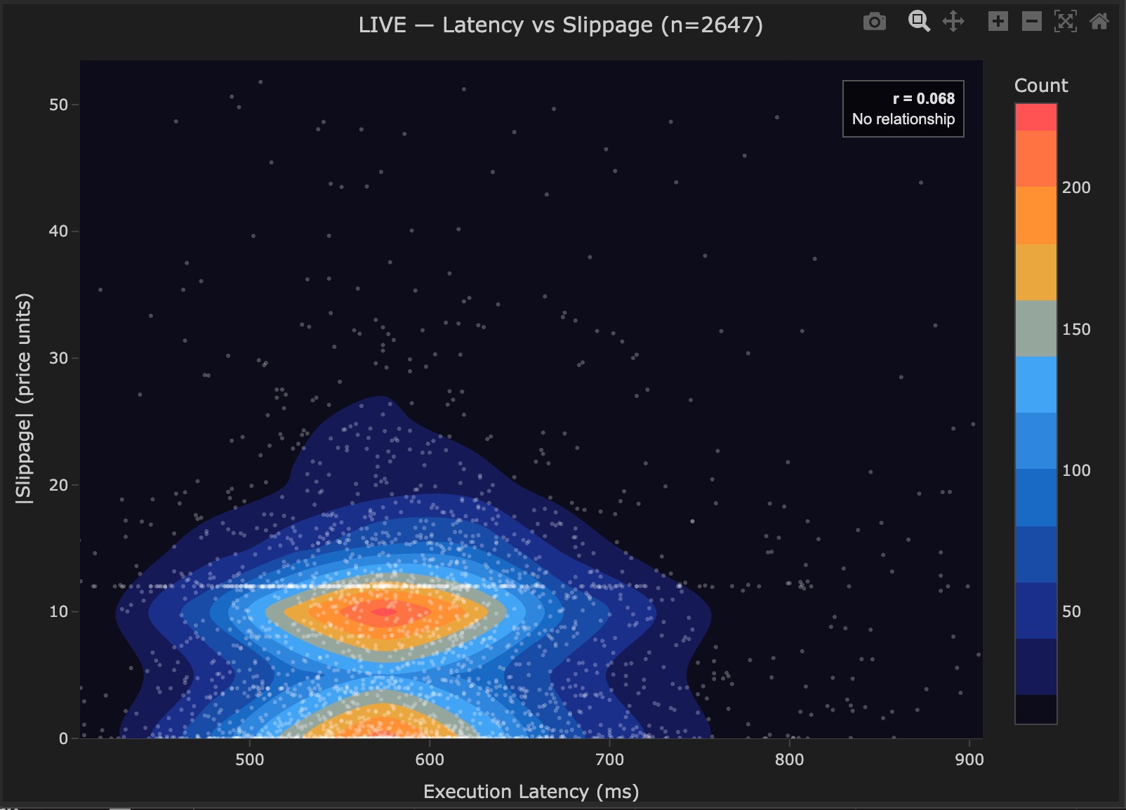
Figure 6: Signal delivery latency vs absolute slippage, n=2,647. r=0.068, no relationship. Two density regions are visible — the upper cluster corresponding to entry fills centered near 12 price units, the lower cluster corresponding to exit fills centered near zero — consistent with the entry/exit asymmetry from Chapter 4.
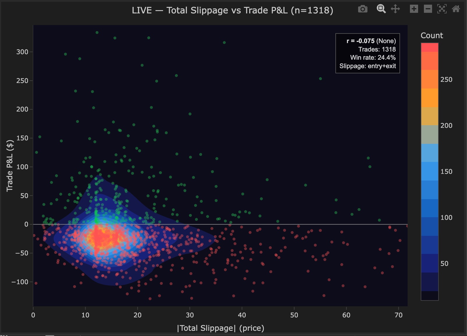
Figure 7: Total absolute slippage vs trade P&L, n=1,318. r=−0.075, no relationship. Winning (green) and losing (red) trades show identical slippage distributions. Win rate 24.4%.
Description of Results
Latency vs Slippage (r=0.068): The density plot shows a horizontal main cluster concentrated between 500 and 700ms and 0 to 25 price units of absolute slippage. The cluster does not tilt upward with increasing latency. Two distinct density regions are visible within the cluster, one centered at approximately 12 price units and one centered near zero, consistent with the entry and exit populations from Chapter 4. The sparse scatter above the main cluster is distributed uniformly across all latency values. The correlation of r=0.068 is classified as no relationship.
Slippage vs P&L (r=−0.075): The density plot shows winning trades concentrated above the P&L zero line and losing trades below it, as expected by definition. Both populations span the same horizontal range of slippage values, approximately 0 to 30 price units for the main cluster. There is no visible separation between winners and losers along the slippage axis. The correlation of r=−0.075 is classified as no relationship. Win rate is 24.4%, confirming the deliberately unprofitable nature of the strategy and providing a clear asymmetry between green and red populations that makes the independence finding directly interpretable.
Interpretation
Latency vs Slippage: The independence of latency and slippage for this strategy confirms that the 581ms median signal delivery time is not a material execution cost driver. For an M1 strategy, a signal delivered anywhere within the 749ms P95 window does not produce measurably different fills from one delivered in 450ms. The market does not move enough within that window, relative to the spread cost, to create a detectable latency effect.
This is an important boundary condition. It applies to M1 and longer timeframe strategies. On sub-minute strategies where signals are generated on seconds-based candles, the relationship between latency and slippage would need to be re-evaluated, as the execution window would represent a larger fraction of the candle's lifetime and price movement within it would be proportionally larger. For the timeframes most systematic retail traders use, the data here provides direct evidence that reducing signal delivery latency below the current 581ms would not meaningfully improve fill quality.
The two density regions visible in Figure 6 are themselves worth noting. They are the direct signature of the entry/exit cost structure, made visible by the high trade count. With 2,647 data points, the underlying execution model becomes structurally visible in the shape of the density plot in a way it would not with 50 or 100 trades.
Slippage vs P&L: The independence of slippage and trade outcome mirrors the latency finding. Just as signal delivery time does not predict fill quality, trade outcome does not predict fill quality either. Slippage is not systematically higher on winning trades or losing trades. The r of -0.075 across 1,318 completed trades is consistent with zero relationship. Execution cost behaves as a fixed structural cost applied uniformly, independent of how the position ultimately resolves.
Conclusion
Both independence findings are null results, and both are informative. Signal delivery latency does not drive fill quality for this strategy type. Trade outcome does not influence execution quality. These findings rule out two categories of execution problems that would otherwise require investigation and mitigation. The execution cost observed in this analysis is a function of market microstructure and broker spread structure. It is not a function of system delays or execution bias.
7. When Execution Costs More: Temporal Patterns
Method
Mean absolute slippage is calculated for every hour/day combination that received at least one trade during the observation period. The heatmap shows which time windows produced elevated mean slippage within this nine-day dataset. With nine days of data, most hour/day cells appear at most once. The results are observations from a single week of trading, not confirmed patterns. They are the correct starting point for ongoing monitoring, not a basis for immediate filtering decisions.
Results
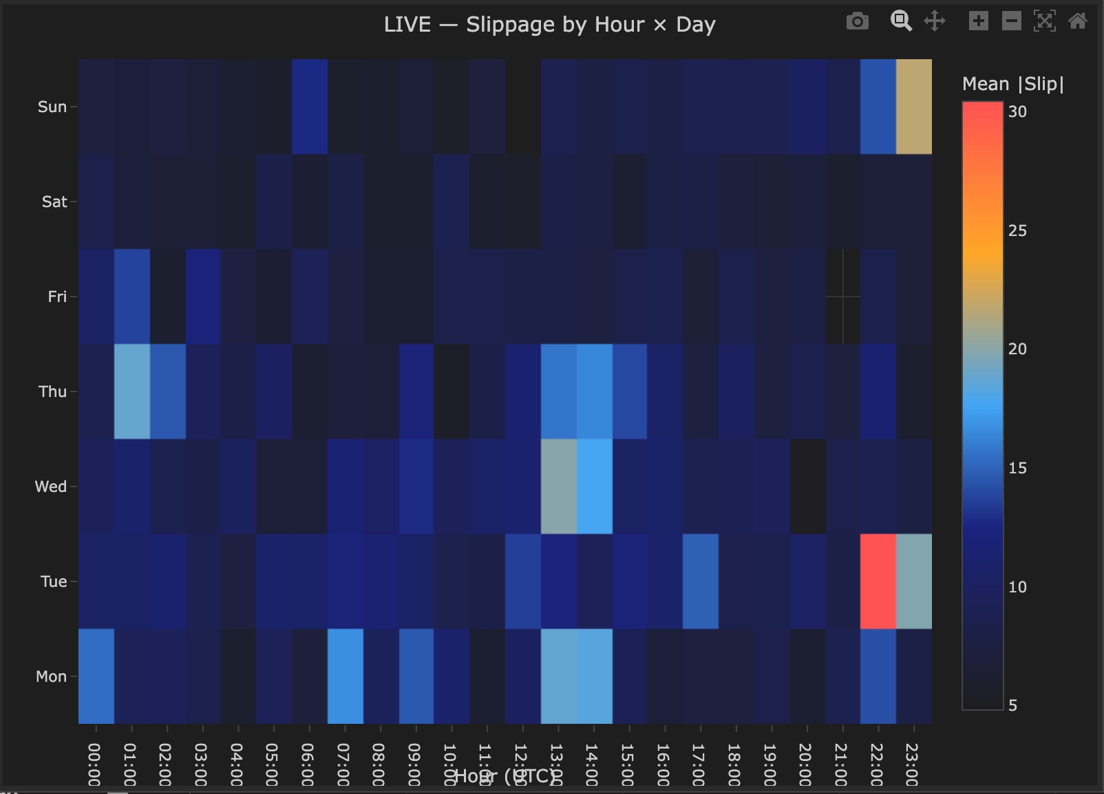
Figure 8: Mean absolute slippage by hour and day, April 1–9. The scale represents mean absolute slippage in price units. The majority of cells are dark blue. Tuesday 22:00–23:00 UTC is the most elevated cell. Wednesday 13:00–14:00 UTC, Thursday 00:00–02:00 UTC, and several other windows show moderate elevation. Empty cells indicate no trades during that period.
Description of Results
The heatmap is predominantly dark blue. The majority of hour/day combinations show mean absolute slippage in the 5 to 10 price unit range, consistent with the spread-driven entry cost identified in Chapter 4.
Several cells stand out. Tuesday 22:00–23:00 UTC is the most prominent, showing the warmest color on the scale. Wednesday 13:00–14:00 UTC shows elevated values. Thursday 00:00–02:00 UTC shows a cluster of elevated overnight cells. Sunday evening 22:00–23:00 UTC shows a warm cell. A small number of additional elevated cells are scattered across the remaining grid.
The Saturday row shows consistently low mean slippage across the cells that appear, consistent with the weekend effect described in Chapter 5.
Interpretation
Nine days of data means most cells represent a single trading session. Tuesday 22:00 UTC appears once. Wednesday 13:00 UTC appears once. A single elevated cell could reflect a genuinely worse execution window, or it could reflect one trade that happened to fill during a momentary price spike. The heatmap cannot distinguish between the two.
What can be said honestly is that the majority of the 24/7 trading week produced execution within the spread-driven baseline. The elevated cells are exceptions, not the norm. The most elevated window, Tuesday 22:00–23:00 UTC, falls in the late US session after main equity and futures activity has wound down and before Asian markets open. Reduced participation during this transition is a plausible explanation for elevated slippage, but one observation is not sufficient to confirm it.
The practical use of this chart is forward-looking. Accumulated over four to six weeks of live trading, the same heatmap will show which cells are consistently elevated across multiple occurrences of each weekday and hour. At that point the data supports a filtering decision. After nine days it supports monitoring.
Conclusion
The temporal heatmap identifies which hour/day combinations produced elevated slippage within this observation period. The majority of trading hours show execution near the spread-driven baseline. Several cells are elevated, with Tuesday 22:00–23:00 UTC the most prominent. None of these observations can be confirmed as structural patterns from nine days of data alone. The heatmap is the right instrument for this analysis. It requires more data to produce actionable conclusions.
8. The Leverage Multiplier: Slippage Cost as a Percentage of Margin
Method
The slippage cost for each entry fill is expressed as a percentage of the broker margin required to open that trade. This normalises execution cost relative to capital committed, making it directly interpretable regardless of position size or account balance. Margin values are sourced from the execution log, where the EA reports actual margin required for each fill via MT5's OrderCalcMargin() function.
Results

Figure 9: Slippage cost as percentage of broker margin per entry fill, n=1,319, reflecting entries with complete broker margin data. Mean 5.1%. The band is stable across the observation period. Outliers above 10% are present throughout and are not clustered at specific times.
Description of Results
The mean slippage cost as a percentage of broker margin per entry fill is 5.1%. The individual fills form a stable band centered on the mean throughout the nine days. The majority of fills fall between 2% and 8% of margin. A scatter of outliers extends above 10%, with isolated points reaching above 20% and a small number above 40%. These outliers are distributed across the full period without clustering at specific dates or times.
For context from the execution log, mean broker margin per trade was approximately $233, and mean position exposure was $68,070. This corresponds to an effective leverage of approximately 250:1 per trade.
Interpretation
The 5.1% figure requires careful interpretation. It does not mean that 5.1% of capital is consumed per trade. It means that the slippage cost on each entry fill is equivalent to 5.1% of the broker margin committed to open that position.
The calculation for a typical trade is straightforward. A 12-unit slippage on 0.82 lots produces a dollar slippage cost of approximately $9.84. Divided by the broker margin of $233, that is 4.2%, consistent with the observed cluster. The mean of 5.1% is slightly above this because individual trades with larger slippage during volatile moments pull the average upward.
At approximately 250:1 effective leverage, a 12-unit slippage on a $68,000 BTCUSD position represents 5.1% of the $233 margin that opened it. At 1:1 leverage, the same 12-unit slippage on the same position would represent 0.018% of capital deployed. The absolute cost is identical. What changes is how it appears relative to the capital at stake. This is the leverage multiplier effect on execution cost.
That number is not directly readable from a broker's pricing page. A quoted BTCUSD spread of approximately 12 price units tells you the nominal cost. It does not tell you the cost relative to the capital you commit at the leverage level your strategy actually uses. The spread as a percentage of margin is a function of the spread, the instrument price, and the effective leverage applied. All three change continuously. Direct measurement from live fills is the only way to arrive at it with confidence, as discussed in Chapter 4.
The outliers above 10% and above 20% are not anomalies requiring explanation. They are fills where BTCUSD price movement during the execution window was large. Price spikes, volatility bursts, or momentary liquidity gaps expanded the fill cost beyond the typical spread range. They are present throughout the period without clustering, consistent with the random arrival of high-volatility moments on a continuously traded 24/7 instrument.
Conclusion
At approximately 250:1 effective leverage on a CFD instrument with spread-inclusive cost structure, the nominal spread of 12 price units translates to approximately 5.1% of broker margin per entry fill. This sits in the moderate range. For a strategy with tight profit targets relative to margin, this cost warrants careful attention in position sizing. For a strategy with a validated edge and wider per-trade return targets, it is a quantifiable and manageable cost. The number does not appear in backtest results, broker fee schedules, or simplified cost model assumptions. Direct measurement from live fills is what makes it observable.
Conclusion
The central question this analysis set out to answer was practical. What do execution costs actually look like, how do they appear, how large are they relative to the capital committed, and can they be reliably modelled? Nine days of live BTCUSD execution data across 2,723 signals provide a direct answer to each part of that question.
Execution costs appear as spread. The slippage distribution makes this structural. The dominant entry bar at 12 price units is not noise. It is the broker spread, made directly readable by the volume of fills. MT5 candles are bid-based and BUY orders fill at the ask. The spread is paid on every entry. The scatter of fills around that peak reflects genuine price movement during the execution window. Exit slippage averages near zero. The cost model of a standard CFD account, with commission embedded in the spread, produces a consistent and interpretable signature in the data. The temporal heatmap shows that this cost is not constant. It has a knowable weekly structure, with most of the trading day near the baseline and a small number of identifiable windows elevated. The signal delivery pipeline is stable throughout, with a near-Gaussian latency distribution at 581ms median that does not respond to market conditions and does not influence fill quality. Neither latency nor trade outcome has any detectable relationship with slippage in this dataset.
The most strategically important finding is the 5.1% of broker margin per entry fill at approximately 250:1 effective leverage. An estimate of this number is possible if you know your effective leverage per trade, your typical spread, and your exact lot sizing after broker rounding constraints are applied. But all three inputs carry uncertainty. Effective leverage is not always the account maximum. A 500:1 account can produce 250:1 effective leverage at a given position size, as this dataset shows. The spread is not a constant. The distribution around the central bar in Figure 4 quantifies exactly how much it varies across fills. And the lot size is discretized to the broker's volume step, introducing a further gap between theoretical and actual. Direct measurement from live fills replaces those estimates with observations and makes the variation visible, not just the mean.
The costs here are deterministic and stable. They are not the result of execution randomness, broker bias, or latency effects. That makes them modelable. A trader who measures them can incorporate them precisely into a position sizing framework. A trader who does not measure them is sizing positions against an assumption that may be systematically wrong.
The preceding article in this series validated a BTCUSD EMA crossover strategy on M30 with a p-value of 0.008 across five out-of-sample windows, including two windows where BTC price was declining. That article established that the strategy has a real edge in the current regime. This article establishes the execution cost structure that any live deployment of that strategy operates within. The next step is to combine a validated edge, a measured execution cost, and an empirical risk envelope from the walk-forward analysis, and derive from that combination how much capital each position should commit.
A deployment hypothesis without that step is incomplete. A 5.1% per-fill cost on broker margin is not an obstacle to deployment. For a strategy with the edge characteristics documented in the WFO analysis, the expected return per trade at appropriate sizing comfortably exceeds this cost. But appropriate sizing cannot be determined without knowing the cost. That is the calculation Article 4 will perform.
Every chart and metric in this report is generated automatically by the Strateda TCA suite. Any trader with a connected MT5 broker account can run the same analysis on their own strategy and broker. The findings here reflect one instrument, one broker, and one nine-day period on a demo account. The methodology applies to any live deployment.
This report is for educational and informational purposes only. It does not constitute investment advice. Past execution quality is not indicative of future results.
This article is part of a research series on the complete strategy lifecycle.
Previous: Walk-Forward Optimization. Validating whether a strategy's edge is real and characterizing the conditions in which it operates.
You are here: Transaction Cost Analysis. Measuring what execution actually costs and why it matters for live deployment.
Next: Position Sizing and Capital Efficiency. Given a validated edge, a measured execution cost structure, and an empirical risk envelope, how much capital should each position commit?