Running Live Algorithmic Strategies at Scale: Signal Delivery and Execution Precision in Production
Measurements in this article reflect specific production deployments over the stated 29-day observation window (March 28 – April 25, 2026). They characterize the observed behaviour of those deployments at those operating points. Performance on individual user deployments and at future points in time may differ materially due to load, network conditions, broker behaviour, account type, and configuration. Past observations of system performance do not guarantee future performance.
Introduction
The gap between a backtest's reported performance and what a live strategy actually delivers has two distinct sources. The first is broker execution: what the broker charges in spread, how slippage distributes around the intended fill price, how those costs compound across hundreds of trades. The previous report in this series, the transaction cost analysis, measured that side of the chain on a single strategy over a 9-day window.
This report measures the other side. Between the moment a strategy generates a trade signal on a cloud server and the moment that signal arrives at the broker for execution, there is a signal delivery pipeline. It runs continuously, serves every active live strategy in parallel, and has to remain stable under whatever load the user runs against it. If the pipeline drops signals, delivers them late, or behaves inconsistently across strategies, no amount of broker-side optimization can compensate.
The question this report answers is whether the pipeline holds up at scale. The primary dataset comes from a production EU deployment that ran 13 live strategies concurrently for 29 days and delivered 59,737 signals. A secondary US deployment running 2 strategies over the same window contributed 16,623 signals; that smaller dataset is used in Chapter 3 to decompose where the latency budget goes, and again in Chapter 5 as a second empirical anchor for the broker-confirmed slippage σ, since the two deployments share the same architecture but differ in concurrent load and broker-execution geometry.
Chapter 1 describes the load: which strategies were running, on what instruments, with what trade frequencies. Chapter 2 describes the architecture and what the design predicts the measurements should look like. Chapters 3 and 4 measure how the system performed: latency and execution precision respectively. Chapter 5 translates the latency measurements into the spread-equivalent cost framework introduced in the TCA report, completing the bridge between system-side and broker-side measurements.
The TCA report validated the broker. This report validates the pipeline that gets signals to the broker. Together they account for the full execution chain.
1. The Setup
The observation period spans 29 days, from March 28 to April 25, 2026. Throughout this window, a single production EU server hosted 13 live strategies running concurrently and routed every trade signal to MetaTrader 5 via the Strateda Expert Advisor. All trading occurred on demo accounts spread across multiple user IDs.
The 13 strategies were chosen to exercise the pipeline across a meaningful range of operating conditions rather than to test a single signal type at high volume. They cover:
- Three instruments with different market structures: BTCUSD (24/7, high volatility), EURUSD (24/5 with weekend breaks, moderate volatility), and EURCHF (24/5 with weekend breaks, very low volatility).
- Two timeframes: M1 (one-minute candles, signals up to every minute) and M5 (five-minute candles, signals up to every five minutes).
- Indicator periods spanning two orders of magnitude, from the fastest configurations (EMA 2/5, generating signals constantly during ranging markets) to the slowest (EMA 20/500, generating signals only on major regime shifts).
- Variant strategy types: Live entries with crossover exits, Live entries with directional filters (Buy-only or Sell-only variants), and Stops variants where exits are governed by explicit stop-loss conditions rather than indicator reversals.
- Multiple user accounts: the same strategy code in some cases runs under different account IDs, providing implicit cross-validation of per-instance behaviour.
The breakdown by strategy and account:
| Strategy | User | Signals | Instrument | Timeframe |
|---|---|---|---|---|
| BTCUSD-M1-EMA-2/5-Live | user-2 | 12,601 | BTCUSD | M1 |
| BTCUSD-M1-Sell-EMA-2/5-Live | user-3 | 11,383 | BTCUSD | M1 |
| BTCUSD-M1-EMA-2/5-Live | user-0 | 11,125 | BTCUSD | M1 |
| BTCUSD-M1-EMA-2/5-Live | user-3 | 10,083 | BTCUSD | M1 |
| EURUSD-M1-EMA-2/5-Live | user-0 | 5,316 | EURUSD | M1 |
| BTCUSD-M1-EMA-2/5-Stops | user-3 | 3,068 | BTCUSD | M1 |
| BTCUSD-M1-EMA-2/5-Stops | user-2 | 3,065 | BTCUSD | M1 |
| BTCUSD-M1-EMA-Buy-20/50-Live | user-2 | 949 | BTCUSD | M1 |
| BTCUSD-M1-EMA-Sell-20/50-Live | user-2 | 948 | BTCUSD | M1 |
| BTCUSD-M1-Sell-EMA-20/50-Stops | user-3 | 531 | BTCUSD | M1 |
| BTCUSD-M1-EMA-20/500-Live | user-0 | 329 | BTCUSD | M1 |
| EURCHF-M5-EMA-DEMA-Buy-Live | user-1 | 170 | EURCHF | M5 |
| EURCHF-M5-EMA-DEMA-Sell-Live | user-1 | 169 | EURCHF | M5 |
Total signals across the 13 strategies on the EU deployment: 59,737. Trade counts vary widely across strategies, from 12,601 on the busiest down to 169 on the slowest. This spread is itself a property of the load mix the pipeline had to handle. High-frequency M1 strategies on volatile instruments generate hundreds of signals per day; slow-period or low-volatility strategies generate fewer than ten. The pipeline serves all of them through the same delivery and execution path.
A separate US deployment ran 2 live BTCUSD strategies (an EMA 2/5 Live variant and its Sell counterpart) over the same 29-day window, contributing 16,623 signals. The US dataset is used in Chapter 3 for the latency analysis. Chapter 4's execution precision analysis uses the EU dataset only.
The remainder of this report treats the EU pipeline as a single system handling the combined 13-strategy load. Chapter 3 pools all signals at the system level for the latency analysis and uses the US dataset to decompose where the latency budget goes. Chapter 4 measures execution precision on a 12-strategy EU subset, with one strategy excluded on methodological grounds explained in that chapter. Chapter 5 translates the system measurements into the spread-equivalent cost framework from the prior TCA report.
2. Architecture
A latency number is only as meaningful as the system it characterizes. Two systems can produce the same 579ms median while behaving very differently under stress. This chapter describes the architecture that produced the measurements in the rest of the report, with enough detail to interpret the numbers honestly.
The system has two halves that meet at a coordination layer.

Figure 1: System architecture. Each live strategy runs in isolation on the server side, backed by persistent state in a coordination layer. A failover monitor restarts any strategy that fails on a healthy instance. Client-side MT5 terminals run the Strateda EA, which polls the coordination layer for pending signals. Measurements were collected at two operating points: an EU deployment (13 strategies, Frankfurt server, Zurich client) and a US deployment (2 strategies, US-East server, NY VPS client).
Server side
Each live strategy runs in isolation, with its own state and resources backed by persistent state in a coordination layer. The coordination layer serves two roles: it holds the durable state of every running strategy, and it acts as the queue of pending signals awaiting client-side pickup.
Strategy instances are not assumed to be permanent. A failover monitor health-checks every running strategy and automatically restarts any that fails. The coordination layer carries the strategy's persisted state across the restart so the strategy resumes from its last checkpoint. The candle during which the failure occurred may be missed; subsequent candles continue normally with no state corruption.
The design intent is simple: a strategy never dies because of an infrastructure event. Failures are expected and handled. The coordination layer is the source of truth; the strategy instances are replaceable.
Client side
The client side is what makes this system more interesting than a typical cloud-only deployment. MT5 terminals run the Strateda EA, which receives signals from the coordination layer and submits orders to the broker. The mapping between EAs, MT5 terminals, and strategies is flexible: a single MT5 terminal can host EAs for multiple strategies, which keeps the client setup simple and is suitable for higher timeframes where added latency is small relative to candle size; multiple MT5 terminals connected to the same broker account can also serve a single strategy in parallel, which reduces signal delivery latency and is appropriate for low-timeframe strategies. The architecture leaves this choice to the user.
The MT5 terminal runs on the user's own infrastructure rather than Strateda's. This is a deliberate design choice with three consequences. First, it keeps order execution under the user's direct control via their own broker account. Second, every trade Strateda opens appears in the MT5 terminal the user already knows, in real time, with fills and positions visible in the familiar broker-facing UI. Third, manual override is preserved at all times: a user can disconnect the EA, close a Strateda-opened position manually, or intervene at the broker level without any coordination with Strateda's infrastructure.
For the EU deployment, the entire client side ran on two consumer Windows machines in the Zurich region, a laptop and a desktop PC sharing a residential broadband connection. Across the two machines, thirteen MT5 terminals ran concurrently, one per live strategy, plus additional terminals for backtesting EAs serving the same accounts. Each terminal is configured to auto-launch on Windows boot, and each EA is configured to start automatically when its terminal opens. After a PC restart (planned or unplanned), the full client-side stack comes back online without manual intervention.
The client side runs on consumer hardware but applies server-grade operational discipline to that hardware. Cloud infrastructure gives you reliable power, reliable network, supervised scheduling, no surprise reboots. Consumer hardware on residential internet gives you none of these by default. The deployment compensates with explicit configuration: every terminal auto-launches on Windows boot, every EA auto-starts with its terminal, every machine is configured to come back fully without manual intervention.
For the US deployment, the client side ran on a single NY-based VPS instance hosting 2 MT5 terminals connected to the same broker as the EU setup. The VPS configuration mirrored the EU machines' auto-launch behaviour for the MT5 terminals themselves.
How signals move
The two halves communicate through polling. The Strateda EA on each MT5 terminal continuously polls the coordination layer for pending signals assigned to its strategy. When a signal is found, the EA picks it up, executes the order through the MT5 broker connection, and writes the confirmation back.
The polling interval is adaptive within bounds. The EA measures round-trip time to the server and shortens the polling interval when the network is stable, down to a floor of 60ms. The floor is deliberate: it caps the EA's request rate against the coordination layer regardless of how fast the network becomes, protecting backend capacity. During the measurements presented here the polling interval was at this 60ms floor with mean RTT of 27ms, so the polling discovery component is bounded above by 60ms and contributes a small, predictable share of total latency.
The polling-based design predicts an approximately Gaussian latency distribution dominated by network and processing variation, with the polling discovery component bounded and small relative to total delivery time.
Polling is also more robust under transient network failures. If a poll fails, the next poll picks up the same pending signal — no retry logic required. It does not require the server to maintain persistent connections to every active EA, which simplifies the server architecture and tolerates clients connecting and disconnecting freely. For setup details on the EA polling architecture and configuration, see the documentation chapters on Expert Advisor Setup and Live Trading Mode.
Measurement geometry
The two deployments measured in this report sit at different points on the same architecture:
| EU deployment | US deployment | |
|---|---|---|
| Server location | Frankfurt | US-East |
| Client location | Zurich (consumer hardware, residential broadband) | NY (VPS) |
| Network RTT (EA → server) | ~27ms | ~18ms |
| Concurrent strategies | 13 | 2 |
| Signal count over 29 days | 59,737 | 16,623 |
Both deployments use the same coordination layer, the same strategy isolation model, the same failover machinery, the same EA polling logic, and equivalent instance classes. They differ in three measurable ways: network geometry, concurrent load on the strategy host, and (for client maintenance) operational discipline. Chapter 3 uses these differences to decompose where the EU deployment's latency budget actually goes.
What the architecture predicts the measurements should show
If the architecture works as designed, three things follow:
- Signal delivery latency should be tightly distributed. The polling interval, network RTT, and coordination-layer access times are bounded by configuration. There is no obvious mechanism for the round trip to vary wildly absent specific failure modes. The shape should be approximately Gaussian dominated by network jitter and per-strategy processing variation.
- Latency should not correlate with strategy identity within a deployment. All strategies share the same delivery path. A signal from a high-frequency BTCUSD strategy and a signal from a low-frequency EURCHF strategy go through the same coordination layer and the same EA poll loop.
- Execution precision should be high but not perfect. Most pending signals should resolve into confirmed broker fills. Some fraction will not: broker rejections, margin conflicts, signals invalidated by position state, network failures during the EA→broker submission step. The failover machinery cannot fix signals that the broker refuses to execute.
The next three chapters test these predictions against 29 days of measurements.
3. System Stability: Signal Delivery Latency
Method
Signal delivery latency is measured for every trade signal across the observation period. The measurement captures the time between signal generation on the strategy server and reception by the MT5 Expert Advisor running on the trader's terminal. Every signal from every live strategy on both deployments is included. Entries (OPEN) and exits (CLOSE) are pooled at this stage; the distribution characterizes the stability of the signal delivery pipeline as a system property rather than the behaviour of any individual strategy.
Total sample size is 59,737 signals on the EU deployment and 16,623 signals on the US deployment across the same 29-day window.
EU results

Figure 2: EU signal delivery latency distribution, 13 concurrent strategies, n=59,737. Median 579ms, P95 777ms, P99 977ms.
The EU distribution is near-Gaussian with a single dominant mode around 560ms and a modest right tail. The median is 579ms, P95 is 777ms, P99 is 977ms. The bulk of the distribution lies between 400ms and 800ms, with the visible right tail extending to roughly 1,000ms before approaching zero. The shape is unimodal throughout — no secondary cluster, no bimodal structure, no heavy-tailed deviation from the central peak.
Per-instance medians and P95s across the 13 strategies fall within a narrow range. The high-volume BTCUSD strategies (n above 10,000) cluster at P50 ≈ 570–580ms and P95 ≈ 750ms. The slower strategies (EURCHF M5, EURUSD M1 low frequency, EMA 20/500) sit slightly higher, at P50 ≈ 615–665ms and P95 ≈ 890–960ms, a difference more consistent with smaller-sample variance than with a systematic instrument effect. The same strategy code running under multiple user accounts produces P50 values that cluster within an 8ms range across instances and P95 values within a 35ms range. Per-instance behaviour is consistent regardless of which user account is running the code.
US results
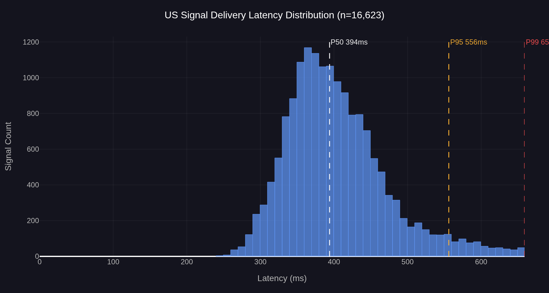
Figure 3: US signal delivery latency distribution, 2 concurrent strategies, n=16,623. Median 394ms, P95 556ms, P99 657ms.
The US distribution has the same shape family — unimodal, right-skewed, no bimodal structure — but sits at substantially lower absolute latencies. The median is 394ms, P95 is 556ms, P99 is 657ms. The bulk of the distribution lies between 280ms and 500ms.
Decomposing the latency budget
The 185ms gap between the EU and US medians is the most informative number in this section. The two deployments share an identical architecture, identical EA code, and identical coordination layer logic. They differ in three measurable ways: network RTT, concurrent load on the strategy host, and client location. The decomposition is:
| Component | EU | US | Difference |
|---|---|---|---|
| Network RTT (EA ↔ server) | ~27ms | ~18ms | ~9ms |
| Concurrent strategies on host | 13 | 2 | factor of ~6.5× |
| Median signal delivery | 579ms | 394ms | 185ms |
Network RTT differences account for at most ~20ms of the 185ms median gap (the polling round trip involves the RTT on the poll request and again on the response, so the network contribution scales roughly as 2 × RTT difference). That leaves ~165ms attributable to per-strategy server-side processing time under concurrent load. The two deployments run on identical server configurations. The only architectural difference between them is the number of concurrent strategies hosted on each.
The implication is that the EU deployment's 579ms median is not a property of the architecture in general; it is a property of this operating point on the architecture. The EU instance was sized to host up to 13 concurrent strategies. Beyond that ceiling, additional strategies are distributed to additional instances of the same class rather than added to existing ones, which keeps per-strategy latency characteristics inside a bounded range as the platform scales. The US measurement, at 2 concurrent strategies on equivalent infrastructure, represents the lower end of the same architecture's operating range.
Interpretation
The near-Gaussian shape on both deployments is the relevant finding, not the absolute numbers. A polling-based delivery system has plausible failure modes that would show up as distinctive distribution shapes: bimodal structure tied to the polling interval, heavy right tail from queuing pressure, periodic spikes from coordination-layer contention or network congestion. None of these are present in either distribution. The single dominant mode with a modest right tail is what is expected from a process dominated by independent random variation. Small jitter around the central polling round trip, rather than systematic intermittent failure, produces this shape.
The 579ms EU median is consistent with the 581ms median measured in the earlier transaction cost analysis on a single strategy over a 9-day window. The current measurement extends that finding by an order of magnitude in sample size, across 13 strategies and three instruments. The system's latency profile is a property of the signal delivery infrastructure at a given operating point, not a characteristic of any individual strategy, instrument, or client account.
The P99 of 977ms on the EU deployment represents the worst-case delivery time for the slowest 1% of signals. For an M1 strategy where each candle represents 60,000 milliseconds, this remains well within the candle window in which the signal was generated. The signal arrives within the first second of the next candle in every case observed during the 29-day window, well before any follow-up signal could fire from the next candle's evaluation. On the US deployment the corresponding P99 of 657ms leaves even more headroom on the same timeframe.
The architecture described in Chapter 2 predicted exactly these profiles: tightly distributed round trips with no instrument or strategy-dependent variation, and shape parameters dominated by network jitter and processing time rather than the polling interval. Both predictions hold across two orders of magnitude of trade frequency, two timeframes, three instruments, two client environments (consumer hardware on residential internet, and a VPS on commercial infrastructure), and 29 continuous days.
Conclusion
Signal delivery latency across both measured operating points was tightly distributed, with the P99 leaving substantial headroom inside an M1 candle window throughout the observation period. The EU production stack, serving 13 concurrent strategies, delivers a median of 579ms with a P99 of 977ms. A lighter-load US deployment on the same architecture delivers 394ms median and 657ms P99. The 185ms gap between the two is dominated by concurrent-load server-side processing rather than network geometry. The two measurements bracket a range of operating points on the same architecture. The remaining chapters examine what happens after the signal arrives at the broker.
4. Execution Precision
Method
Execution precision is the second dimension of signal delivery quality, distinct from latency. Latency measures how fast a signal reaches the broker. Precision measures whether the broker confirms an execution for the signal that was sent. The two dimensions are independent. A signal can be delivered quickly and not result in a fill, or arrive slowly and execute correctly.
For each strategy, the measurement replays the most recent 30 signals produced by the strategy's backtest model and compares each one to the live trade record in the signal delivery table. A signal is considered matched if a corresponding live trade exists within a tolerance of one timeframe window: 60 seconds for an M1 strategy, 300 seconds for M5, and so on. The tolerance matches the system's own behaviour: the live execution engine attempts to fill any signal that did not produce an immediate live trade within the same one-timeframe window. Beyond that window, the signal is considered stale and is not retried. The result is stored as a single record containing the matched count, the total count, the resulting execution rate, and the timestamps of the first and last signal in the 30-signal window.
Each measurement records the execution rate over the most recent 30 signals rather than over a fixed time window. Consecutive measurements share most of those signals, with only the newest entering the window and the oldest rolling off, so the precision time series is autocorrelated. A single non-execution affects multiple consecutive records until it rolls off the 30-signal window. The practical consequence is that a visible dip in the over-time chart represents a sustained execution problem, not a single missed trade.
Non-matched signals are not attributed to a specific cause in this report. The unmatched portion can arise from broker rejection, margin or liquidity constraints, position state conflicts, network failures, or expired signal validity. Two additional contributors specific to this measurement environment are worth naming. First, the live and backtest runs do not share identical start and end boundaries, so a small number of signals at the dataset edges are unmatched simply because the backtest did not generate a corresponding expected trade at that moment. Second, the measurements run against MT5 demo accounts, and demo accounts on most brokers receive lower execution priority than live accounts; this contributes a baseline delay component not present in real-money execution. The aggregate rate is the system property of interest. Per-cause attribution is out of scope.
The precision analysis in this chapter uses the EU deployment only. The US deployment runs the same strategy code on the same broker; using a single deployment for the precision analysis keeps the comparison across strategies clean and isolates strategy-and-instrument effects from cross-deployment differences.
Strategy selection for precision analysis
Twelve of the 13 EU strategies are included; one strategy is excluded on methodological grounds.1 The 7 BTCUSD strategies and the 2 EURCHF strategies, together with 3 additional BTCUSD strategy-account instances of the same code, give 12 strategy-account instances analysed across 32,049 precision windows.
Results
Per-strategy precision results:
| Strategy | User | Windows | Aggregate Rate | Min Window | Max Window |
|---|---|---|---|---|---|
| BTCUSD-M1-Sell-EMA-20/50-Stops | user-3 | 2,747 | 94.6% | 83.3% | 100.0% |
| BTCUSD-M1-EMA-2/5-Live | user-3 | 2,752 | 93.4% | 56.9% | 98.3% |
| BTCUSD-M1-EMA-2/5-Live | user-2 | 2,752 | 93.3% | 53.4% | 98.3% |
| BTCUSD-M1-EMA-2/5-Stops | user-2 | 2,751 | 93.2% | 76.7% | 100.0% |
| BTCUSD-M1-EMA-2/5-Stops | user-3 | 2,752 | 93.2% | 73.3% | 100.0% |
| BTCUSD-M1-Sell-EMA-2/5-Live | user-3 | 2,752 | 93.0% | 57.6% | 98.3% |
| BTCUSD-M1-EMA-2/5-Live | user-0 | 2,710 | 92.4% | 5.0% | 98.3% |
| BTCUSD-M1-EMA-Buy-20/50-Live | user-2 | 2,751 | 91.1% | 77.6% | 98.3% |
| BTCUSD-M1-EMA-Sell-20/50-Live | user-2 | 2,747 | 91.0% | 78.0% | 98.3% |
| BTCUSD-M1-EMA-20/500-Live | user-0 | 2,753 | 88.9% | 76.3% | 95.0% |
| EURCHF-M5-EMA-DEMA-Buy-Live | user-1 | 2,292 | 87.9% | 72.2% | 97.5% |
| EURCHF-M5-EMA-DEMA-Sell-Live | user-1 | 2,290 | 87.3% | 72.2% | 95.0% |
Mean execution rate across 32,049 rolling-window measurements: 91.7% (median 93.2%, P05 79.6%).
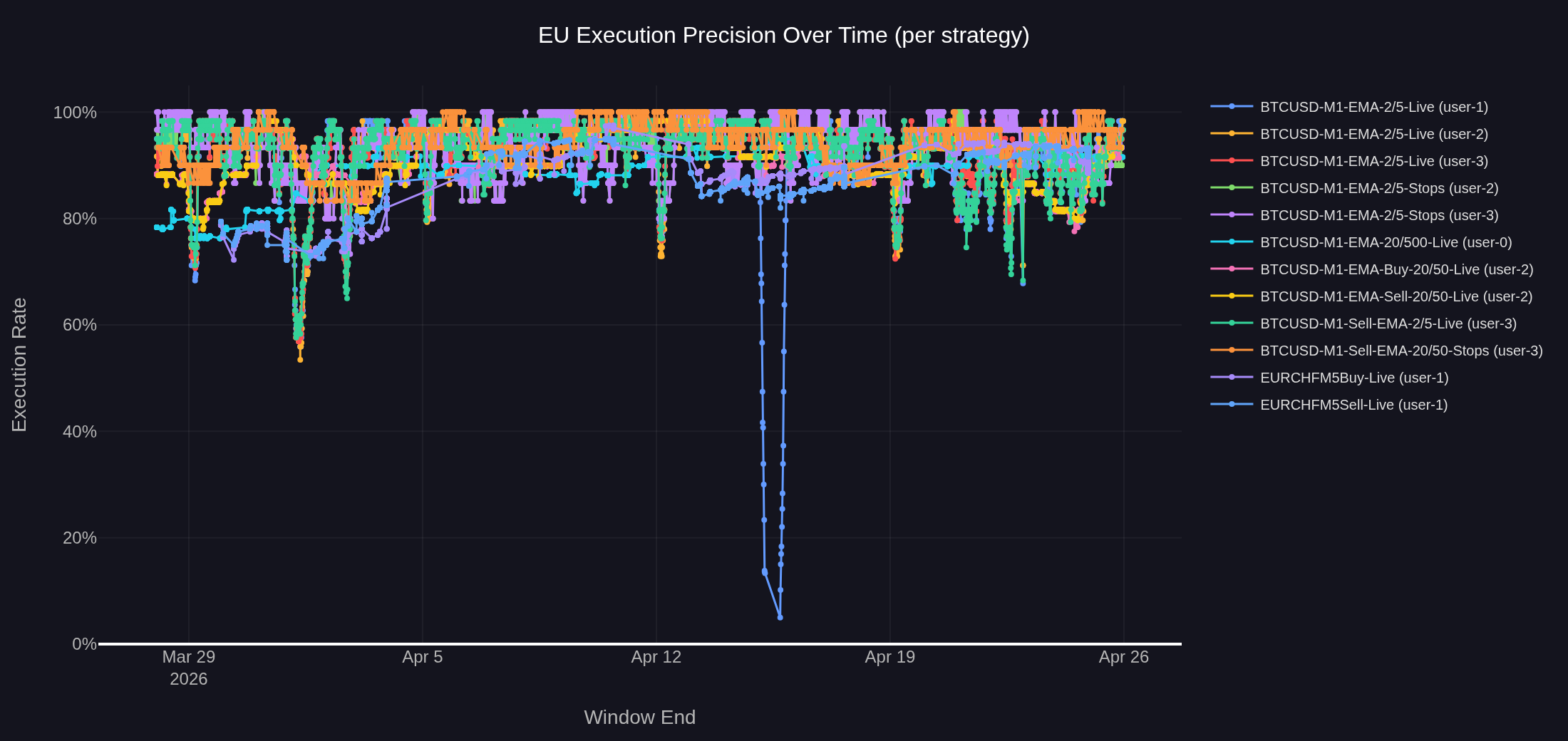
Figure 4: Execution precision over time for the 12 strategies on the EU deployment. Each point represents the match rate over the most recent 30 signals at the time of measurement. Most strategies hold a 85–95% band; one strategy-instance shows a deep isolated dip in mid-April.
The 12 strategies span an 87.3% to 94.6% range, with a system-wide mean execution rate of 91.7% across 32,049 rolling-window measurements (median 93.2%, P05 79.6%). Most strategies hold a 85–95% precision band for the majority of the measurement window.
The data partitions into two clusters. The BTCUSD cluster covers 88.9% to 94.6% across 10 strategy-account instances, a 5.7 percentage point spread. The same strategy code running under multiple user accounts produces aggregate rates within 1.0 percentage point of each other (for example, BTCUSD-M1-EMA-2/5-Live aggregates at 92.4%, 93.3%, and 93.4% across three accounts). This collapses the per-account variation to negligible: precision is a strategy-and-instrument property, not an account-specific one, and the shared infrastructure path is the constant.
The EURCHF cluster sits roughly 5 percentage points below the BTCUSD cluster at 87.9% and 87.3%, the buy and sell variants of the same EMA/DEMA crossover running under the same account. Several instrument-level factors contribute: EURCHF is the only M5 strategy in the analysis and M5 straddles weekend session boundaries more visibly than M1; the strategies run 24/7 and EURCHF liquidity drops sharply during overnight hours when fills can fail entirely or be substantially delayed; and EURCHF has materially lower broker liquidity than BTCUSD even during active hours.
Figure 4 also shows a small number of visible dips below the steady-state band. The deepest isolated drops (the early dip to ~50% and the later drop close to 0%) are attributable to client-side operational events: a terminal disconnection, a terminal restart, a manual disconnection, or a broker connection drop on a single account. The latency data in Chapter 3 shows no concurrent disruption during these events, ruling out a server-side delivery failure. The sub-90% dips visible on the higher-frequency strategies share the same mechanism as the excluded EURUSD-M1-EMA-2/5-Live case: many signals in a short time on a low-volatility instrument produce signal-on-signal conflicts where the broker has not yet confirmed fill on signal N before signal N+1 fires. Neither dip type is an infrastructure event.
The P05 of 79.6% provides the planning baseline for worst-case execution windows: the measured deployment delivered at least four executions out of five even in its worst observed 30-signal windows during the observation period. The 7.3 percentage point spread across strategies is small relative to the 91.7% baseline. The infrastructure path is the constant; observed variation is attributable to strategy-instrument interactions and isolated client-side events, not to architectural failure.
5. Lessons for Live Deployment
The measurements in the preceding chapters answer a system-side question. The signal delivery pipeline is stable at both measured operating points. The EU deployment, serving 13 strategies, delivers a 579ms median with a P99 of 977ms. The US deployment, serving 2 strategies on equivalent infrastructure, delivers a 394ms median with a P99 of 657ms. Execution precision on the EU deployment sits at 91.7% across 12 strategies. The reliability architecture held through the visible incidents.
The relevant question for a reader running their own strategies is whether numbers like these are operationally meaningful for them. The answer depends on two things: the timeframe of the strategy, and which operating point on the architecture the deployment sits at.
Latency as a fraction of the candle
Latency is only relevant relative to the duration of the candle on which the strategy operates.
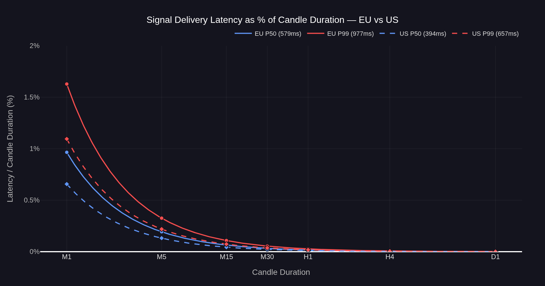
Figure 5: Signal delivery latency as a percentage of candle duration for both operating points. The ratio is latency divided by candle duration — a 1/x curve that decays toward zero as the candle grows. The difference between operating points is most visible on M1 and narrows progressively at longer timeframes.
For an EU M1 strategy, the P99 latency of 977ms occupies 1.63% of the candle. The signal arrives well before the next candle opens in every observed case. For an M5 strategy, the same P99 latency is 0.33% of the candle — operationally negligible. By H1, the worst-case latency is below 0.03% of the candle window.
The US operating point sits below the EU curve at every timeframe, but the difference is only practically visible on M1 (P50 0.66% vs 0.97%, P99 1.10% vs 1.63%). By M5 both operating points are below 0.35% at the P99 level, and by H1 both are below 0.05%. The choice between operating points matters most for the fastest timeframes and disappears for strategies running on M5 and above.
From candle fraction to spread-equivalent drift
The fraction-of-candle view is useful but abstract. A more direct way to size the impact is to express it in the same units the broker charges in — spreads.
The prior transaction cost analysis measured two quantities on M1 BTCUSD entries at the EU operating point. The structural spread came in at approximately 12 price units per fill, a deterministic cost reflecting the bid-ask crossing. The 1σ scatter around that spread came in at approximately 11.35 price units (midway between TCA's entry σ = 11.73 and exit σ = 10.97), a random component reflecting the price movement that occurred during the fill window: the latency-induced drift.
The slippage σ deserves a moment of attention because it does a lot of work in this analysis. Slippage is measured as the difference between the broker-confirmed fill price and the signal price. By construction it captures the price movement during the entire fill window — from the moment the strategy generates the signal to the moment the broker confirms the fill. That window includes both halves of the execution chain: signal delivery (server → EA, measured directly in Chapter 3) and broker execution (EA → broker fill confirmation, measured directly later in this chapter). The σ captures both. That property turns out to matter.

Figure 6: Slippage distribution from the prior TCA report, EU operating point (reproduced for reference). Entry fills (green) centered at +12 price units — the structural spread — with 1σ scatter of 11.73. Exit fills (red) centered at 0 with 1σ scatter of 10.97. The mean of each distribution is the deterministic cost; the standard deviation around it is the random component, capturing price movement during the full fill window — signal delivery plus broker execution.
Empirical anchor at the US operating point
The prior TCA measurement provides the EU drift σ of ~11.35 price units. The US deployment provides a second empirical anchor. Repeating the same slippage measurement on the US setup over a comparable sample (n=1,218 entries, n=1,214 exits) gives an entry distribution centered at +12.00 with σ=6.53, and an exit distribution centered at 0 with σ=6.28 — a measured 1σ drift of ~6.40 price units. The structural spread (12 units, paid on entry) is identical between the two operating points, as expected — that is an instrument property. What differs is the drift σ, which falls by 43% between the EU and US operating points.
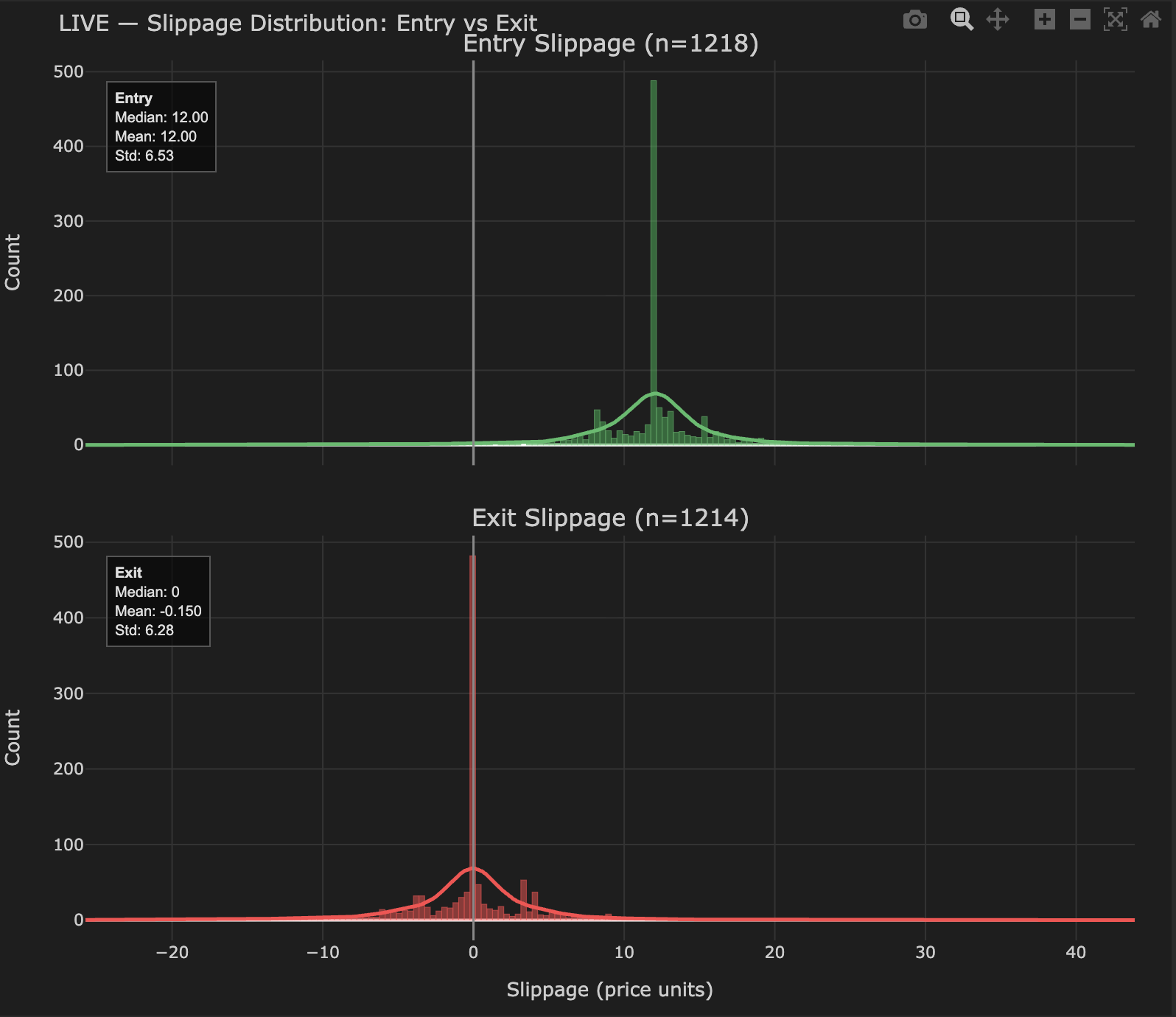
Figure 7: Slippage distribution at the US operating point. Entry fills (green) centered at +12.00 with σ=6.53. Exit fills (red) centered at 0 with σ=6.28. The structural spread is identical to the EU measurement (Figure 6) — same instrument, same broker cost model. The drift σ is roughly half. Combined drift σ across entry and exit is approximately 6.40 price units, down from ~11.35 at the EU operating point.
Direct measurement of the broker execution leg, isolated from signal delivery, makes both halves of the fill window visible. Figures 8 and 9 show the distribution of time between signal arrival at the EA and broker fill confirmation, for the EU and US operating points respectively.

Figure 8: Broker execution latency distribution at the EU operating point. The interval measured is from signal arrival at the EA to broker fill confirmation, isolating the broker execution leg from the signal delivery leg measured in Chapter 3. The modal peak sits at 317ms with P50 of 326ms; the right tail is heavy, with P95 at 13.6s and P99 at 20.6s. The heavy tail is consistent with demo-account broker priority and is not a property of the Strateda signal delivery system.
The US distribution shows the same structural shape — tight modal peak, heavy right tail — shifted leftward by the lower-latency operating point.

Figure 9: Broker execution latency distribution at the US operating point. Same measurement convention as Figure 8. The modal peak sits at 267ms with P50 of 269ms; the right tail follows the same demo-account broker-priority pattern as the EU distribution, with P95 at 13.2s and P99 at 20.0s. Modal-peak execution is ~57ms faster than at the EU operating point.
A pure signal-delivery-latency explanation would predict the σ to scale as √(latency_US / latency_EU) = √(394/579) ≈ 0.825, or a 17% drop. The observed drop is 43% — substantially larger. The remaining gap is attributable to broker-side execution latency, which can be measured directly as the time between signal arrival at the EA and broker fill confirmation. Direct measurement gives a modal peak of 317ms at the EU operating point (P50 = 326ms) and 267ms at the US operating point (P50 = 269ms). Both operating points show a tight modal peak with a heavy right tail extending past 20 seconds at P99. The heavy tail is consistent with demo-account broker priority: demo orders are typically deprioritized when the broker's order servers are busy. The slippage σ observed here, and particularly the heavy right tail in the broker execution distribution, both partly reflect this demo-account priority effect. On live broker accounts, where demo deprioritization does not apply, both the execution tail and the resulting slippage σ are expected to be materially tighter. Direct measurement of this effect on live accounts is a natural follow-up. Both halves of the fill window — signal delivery and broker execution — contribute to the slippage σ, and direct decomposition of which dominates is deferred to a future TCA update.
The slippage σ measures the total fill-window cost. Chapter 3 measures the signal delivery half directly. The new broker-execution measurement (Figures 8 and 9 above) measures the second half directly. The three views are complementary: Chapter 3 isolates what the Strateda architecture controls, the broker execution figures isolate what the broker contributes, and the slippage σ captures the price cost of both halves combined.
Drift as a fraction of the candle
What changes across timeframes is the candle's natural price movement. Short-term price movement is conventionally modeled as a random walk, with the magnitude of price movement over a time window scaling as the square root of that window's duration. The candle's typical 1σ price move grows with √candle_time, so the same drift σ — fixed for a given operating point — becomes a progressively smaller fraction of what the strategy is naturally trying to capture.
Anchoring on the empirically measured σ values (11.35 EU, 6.40 US) and the EU M1 drift fraction calibrated from the prior TCA work, the per-timeframe drift fractions are:
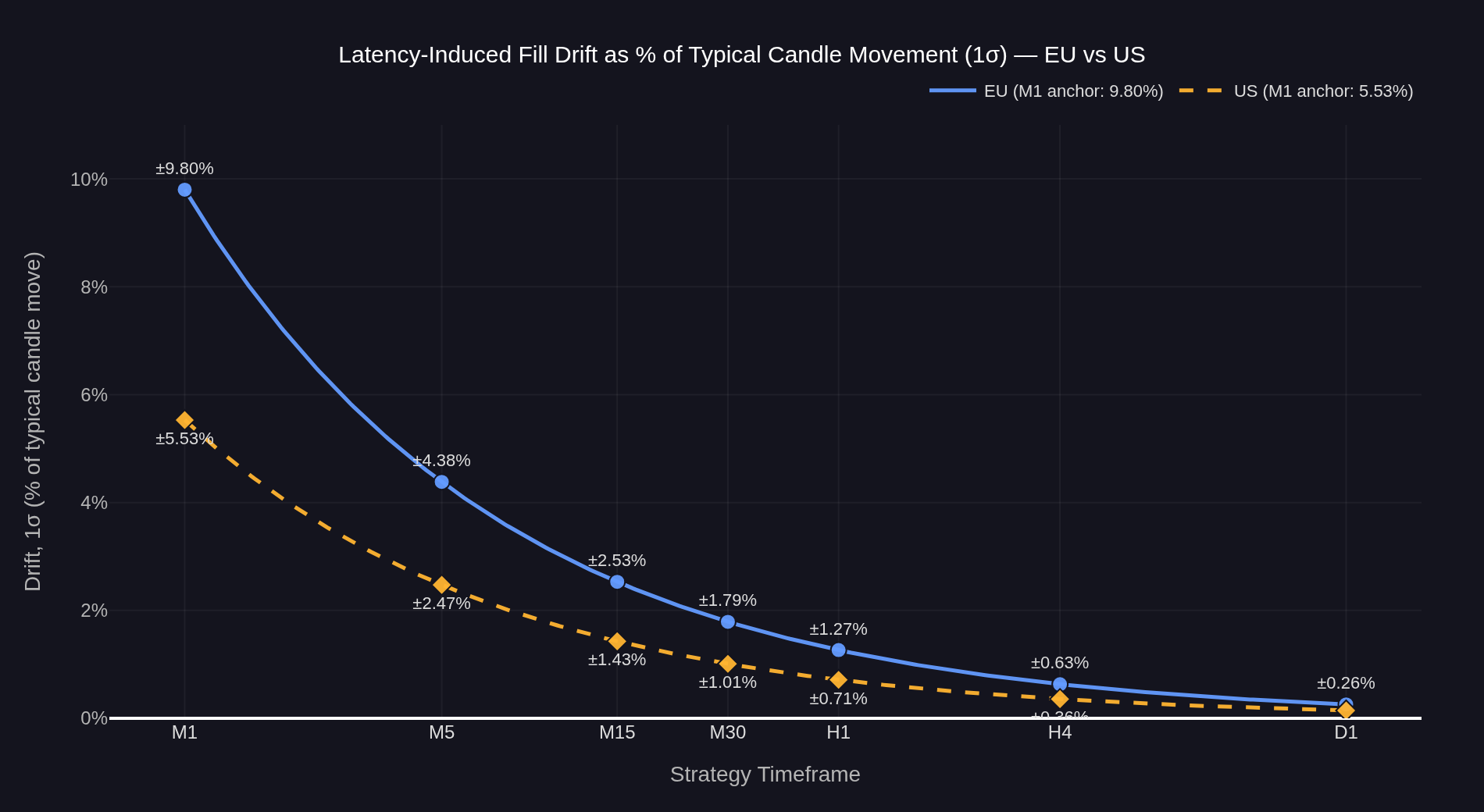
Figure 10: Latency-induced drift, 1σ, expressed as a percentage of the candle's typical natural price movement, for both operating points. Anchored on the empirically measured slippage σ from Figure 6 (EU, σ=11.35) and Figure 7 (US, σ=6.40). Under random-walk scaling, the candle's 1σ price move grows with √timeframe while the measured drift σ stays fixed at a given operating point, so the ratio falls as √(1/candle_time) at each operating point. Drift is symmetric around zero — each fill can be improved or worsened by this amount with equal probability.
At the EU operating point: on M1 the drift is ±9.8% of the typical candle move (1σ), on M5 ±4.4%, on M15 ±2.5%, on M30 ±1.8%, on H1 ±1.3%, on H4 ±0.6%, on D1 ±0.3%.
At the US operating point: on M1 ±5.5%, on M5 ±2.5%, on M15 ±1.4%, on M30 ±1.0%, on H1 ±0.7%, on H4 ±0.4%, on D1 ±0.2%.
Three things follow and matter together. First, the drift is symmetric: each individual fill is equally likely to be improved or worsened. Across many trades the average effect is zero — latency does not systematically move P&L in either direction. What latency drift does affect is per-trade variance: a higher drift σ widens the distribution of per-trade outcomes around the same mean, which compresses Sharpe ratio. Timeframe choice matters precisely because of this: at M1, drift σ may be comparable to the strategy's expected per-trade move and materially compress Sharpe; at H1, drift σ is small relative to candle volatility and execution noise is operationally negligible. Second, the per-fill uncertainty is real, and its significance relative to the strategy's natural price movement falls sharply with longer timeframes. At the EU operating point the drift is roughly a tenth of the natural candle move on M1, a 25th by M5, a hundredth by H1, a four-hundredth by D1 — operationally invisible against the move the strategy is trying to capture. Third, the choice of operating point matters significantly on M1 — the US setup reduces M1 drift from ±9.8% to ±5.5% of the typical candle move, a 44% reduction — but the gap narrows quickly with longer timeframes. By M30 the gap is roughly 0.8 percentage points; by H1 it is below 0.7 percentage points; by H4 it is invisible.
What this implies for deployment
The two measurements bracket the architecture's operating range. The EU deployment runs at its calibrated capacity ceiling for the instance class, hosting 13 concurrent strategies and delivering a 579ms median signal delivery latency. The US deployment, at 2 concurrent strategies on equivalent hardware, sits at the lighter-load end of the same range and delivers 394ms median signal delivery. The slippage σ on the broker-confirmed fills compounds these differences with the broker-execution leg, giving total fill-window drift σ of 11.35 (EU) and 6.40 (US).
The practical implication is timeframe-dependent. For M1 strategies the operating point matters substantially — the drift fraction nearly halves at the US operating point, and the strategy designer has a real decision to make about which deployment configuration is appropriate for their timeframe. For M5 strategies the gap narrows to about 2 percentage points of candle move. By M30 the difference is below 1 percentage point. By H1 and above the difference between the two measured operating points falls below 0.05% of candle duration, a magnitude small relative to typical candle-level price movement.
This connects the two reports. Signal delivery latency, measured in this article, is the first step of the execution chain. Broker-side latency and slippage, measured in the prior TCA report, is the second step. The total fill-window drift σ is the single broker-confirmed measurement that captures both. The first step is bounded, predictable, and tunable by operating point; the second step is where the dominant cost lives and where attention should be focused for strategies running on M5 and above.
Conclusion
System stability is not the absence of failure. It is the presence of bounded, predictable variation in the face of failures that will inevitably occur.
Across 29 days, the primary EU production deployment served 13 live strategies on three instruments and two timeframes at a 579ms median signal delivery latency, with the slowest 1% completing within 977ms and execution precision sitting at 91.7%. The same architecture, measured at a lighter-load operating point in a US deployment, delivered 394ms median signal delivery latency over 16,623 signals across the same window. The two most prominent precision dips in the EU window were diagnosable: one strategy-specific (EMA 2/5 signal conflicts on BTCUSD during a ranging regime), one account-specific (an isolated single-account event lasting about a day). Neither was a server-side infrastructure failure. The shared delivery path held throughout.
These properties are not free. They are the measurable consequence of explicit design choices: per-strategy isolation on the server side, automatic failover with persistent state, polling-based delivery that tolerates client-side network interruptions, adaptive polling intervals bounded by a deliberate floor, client-side auto-launch configuration that survives Windows restarts. The architecture in Chapter 2 was built to produce exactly this kind of bounded, predictable behaviour under load. The data in the chapters that follow confirms it did — at both operating points where it was measured.
The total fill-window cost, captured directly by the broker-confirmed slippage σ, drops 43% from 11.35 price units (1σ) at the EU operating point to 6.40 at the US operating point. Both faster signal delivery and closer broker-execution geometry contribute. Translated to the candle the strategy operates on, this puts M1 drift at ±9.8% of the typical natural move at the EU operating point and ±5.5% at the US operating point. By M5 these numbers fall to ±4.4% and ±2.5%. By M30 both are at or below ±2%. By H1 and above the difference between the two measured operating points falls below 0.05% of candle duration, a magnitude small relative to typical candle-level price movement.
The infrastructure layer is not what limits live performance for the strategy classes Strateda customers run on M5 and above. For M1 strategies the operating point is a real design decision with quantifiable trade-offs. For everything slower than M1, the dominant costs sit further downstream, in broker spread and execution. The prior TCA report already characterized those costs in detail.
The two reports together account for the full execution chain. The pipeline that gets signals to the broker is bounded, predictable, and characterized across the architecture's operating range. The broker that fills those signals is the larger cost. The slippage σ is the single measurement that captures their combined effect. Both halves of the chain are measurable. Both are now measured.
See Terms & Conditions for the scope of the service.